How to use the Array Formula in Google Sheets

The ARRAYFORMULA function in Google Sheets allows you to apply a formula you use in one cell across an entire column. This means you don’t have to copy-paste or drag the formula across the cells where it has to be used, which can be handy when you have a lot of cells to cover. Thus, you can apply formulas across multiple ranges and automate calculations that would otherwise take a lot of time and you can even use it with other functions like IF, SUM, and SUMIF.

Using the Array Formula

The syntax for the function is ARRAYFORMULA(array_formula) and you can use it where only a single argument is needed. This can include a function for multiple similar-sized arrays, an expression, or a cell range. You can use the function when you’ve already entered the formula or when you want to focus on the formula and use the Array Formula function later.

1. For instance, we need to perform a multiplication for the Quantity Sold with the Unit Price in the example here.

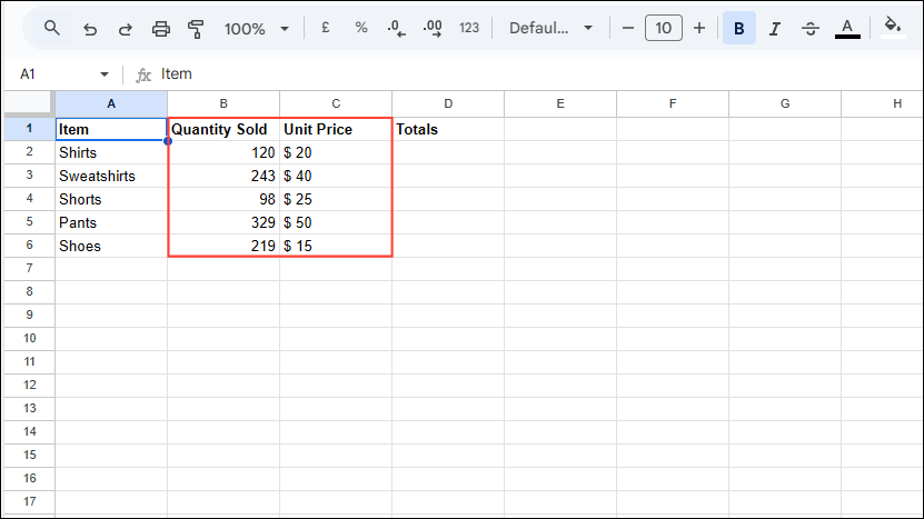
2. The formula that you need to use here will be =ARRAYFORMULA(B2:B6*C2:C6) that will multiply the cells from B2 through B6 and from C2 through C6.

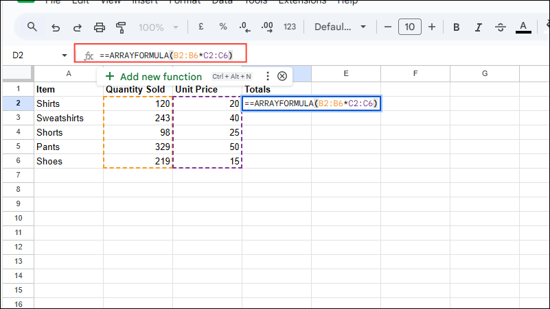
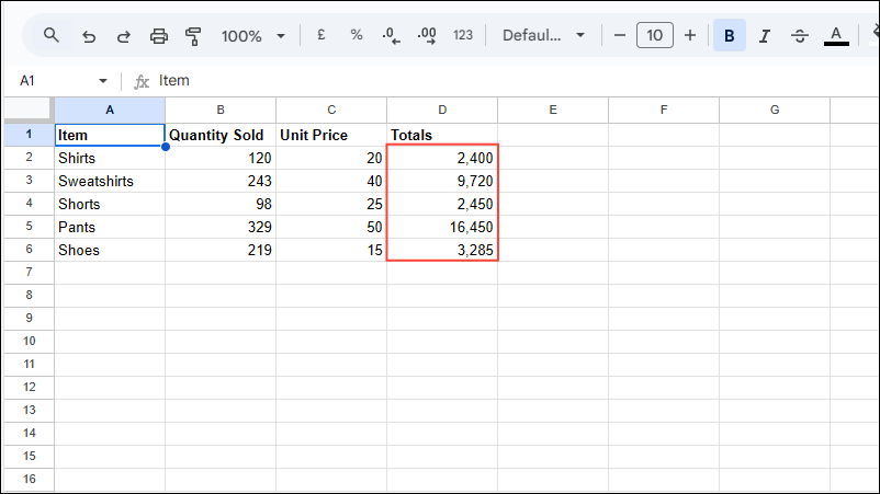
3. When you press Enter, you will see the product of the Quantity Sold and Unit Price columns in the Totals column.

Using the IF function

As mentioned before, you can use the Array Formula with other functions, like the IF function as the argument.

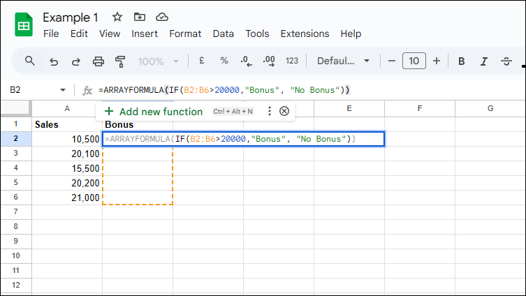
1. In this example, we will use it to show ‘Bonus’ if the amount in the specified cell range exceeds 20,000 and ‘No bonus’ if it does not.

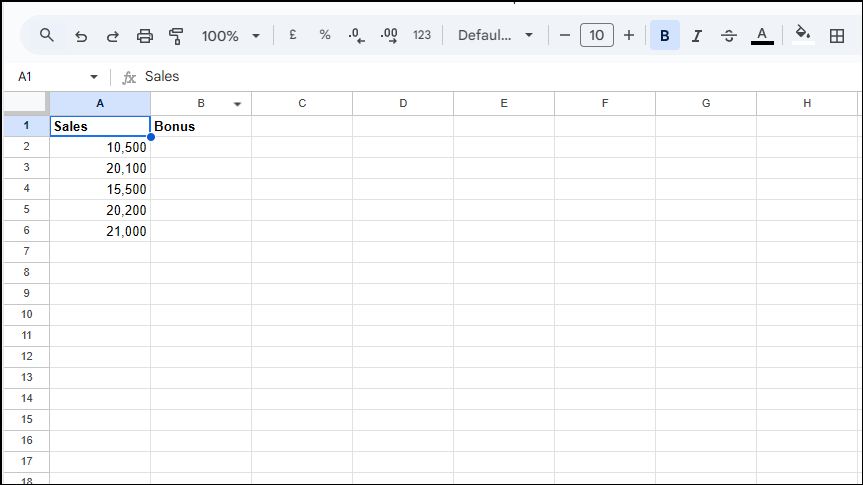
2. The formula will be =ARRAYFORMULA(IF(B2:B6>20000,"Bonus", "No Bonus")). This will generate the output for the entire range.

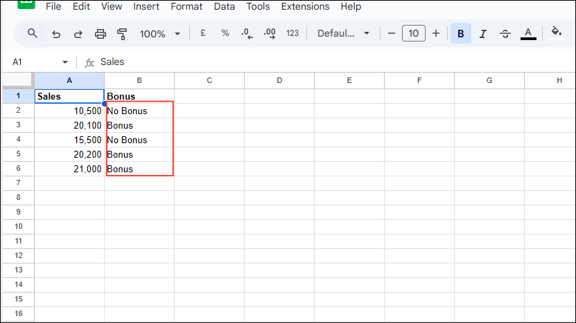
3. Press Enter and you will see the output in the bonus section.

Using the SUMIF function

You can also use the SUMIF function with Array Formula.

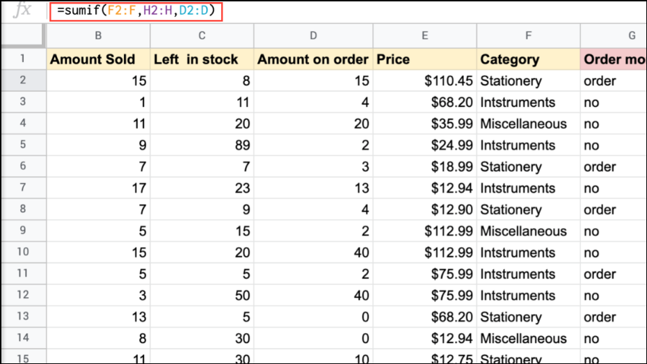
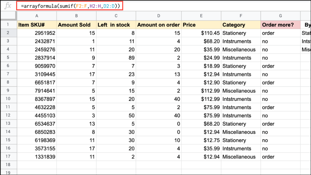
1. In this example, we need to find out the number of stationery items ordered using the SUMIF function. The formula will be sumif(F2:F, H2:H, D2: D).

2. Pressing Enter will show you the output as 32 in cell I2.

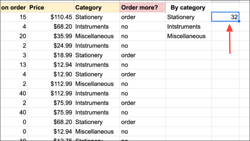
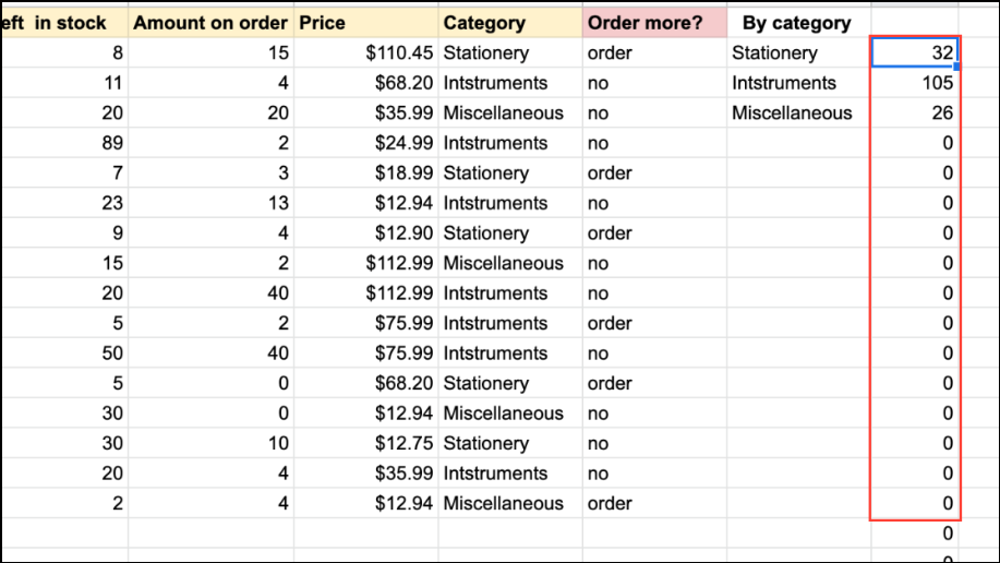
3. Now, you can use the Array Formula to determine the number of items ordered for every category using =arrayformula(sumif(F2:F,H2:H,D2:D).

4. Pressing Enter will show you the output.

Things to know

• When using the Array Formula, make sure that each array is of the same size.
• You can use the Ctrl + Shift + Enter shortcut to add ‘ARRAYFORMULA’ at the beginning of the formula automatically.
• When you make changes to a single cell using the Array Formula, it will take place across all the cells in the range.
• While the Array Formula works with several other functions in Google Sheets, it does not work with Query or Filter functions.