Microsoft Excel is perhaps the most famous program used for managing and analyzing data. You can use it to organize, calculate, and format data, but not many people know that you can even translate languages and detect the language in a workbook in the application.
This is possible thanks to the TRANSLATE and DETECTLANGUAGE functions, which were added to various versions of Excel in December 2024. You can access these functions in the desktop version of the program on Windows and Mac, the mobile app (only for Microsoft 365 subscribers), and the web.
Syntax of the TRANSLATE function
There are three arguments to the TRANSLATE function: =TRANSLATE (a, b, c).
a: This refers to the text to be translated and is placed within double quotes. Alternatively, it may contain the cell reference of the cell containing the text you want to translate.
b: This contains the code of the source language and is also placed within double quotes. It is an optional argument, so if you don't include it, Excel will try to detect the language automatically. That said, if you know the language and its code, you should always include it as it will help in making the translation more accurate.
c: This will contain the target language within double quotes. If you don't include this argument, Excel will automatically consider your system language as the target language. In this case also, including the argument will ensure better translation.
Syntax of the DETECTLANGUAGE function
The DETECTLANGUAGE function contains just one argument: =DETECTLANGUAGE (x), where 'x' is placed within double quotes and is the language to be detected or the cell reference of the cell containing the language to be detected.
To use either of these functions, you will need to know the language code of the languages that are being used. The language code for English is 'En', Russian is 'Ru', Spanish is 'Es', and French is 'Fr'. You can find other language codes on Microsoft's website.
Using the TRANSLATE function
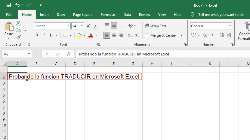
- Open a new Excel worksheet and paste the text you want to translate into any cell. Here, we've pasted the text in Cell A2.
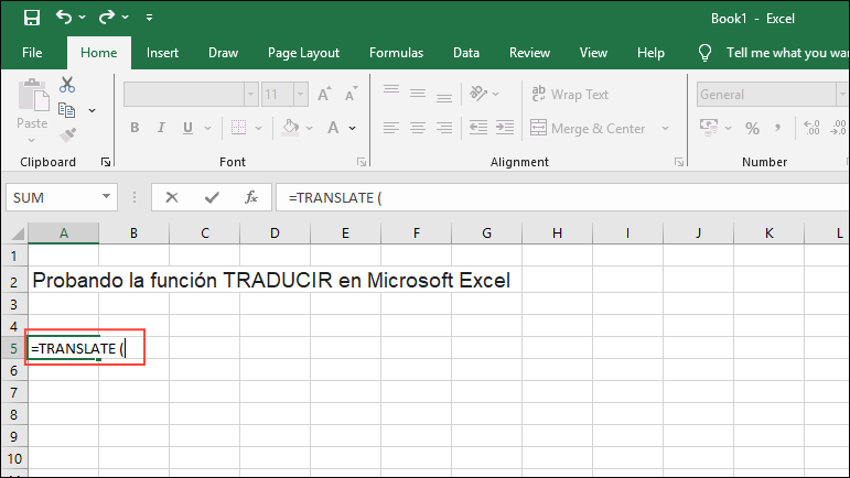
- Now go to another cell (where you want the translation to appear) and type
=TRANSLATE(.
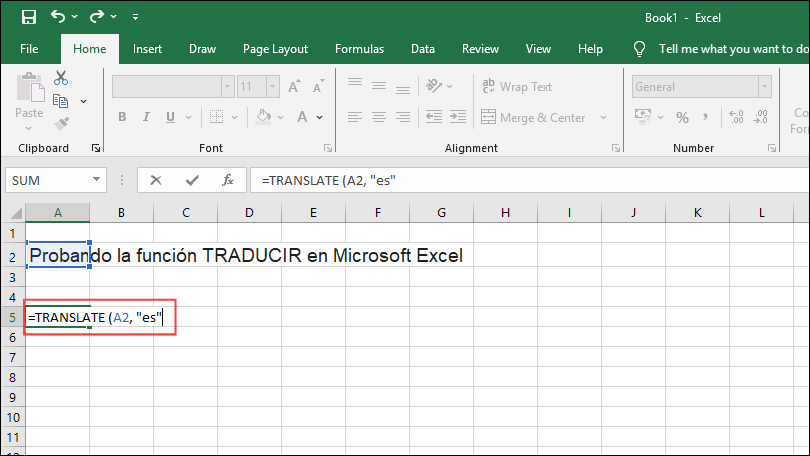
- Enter the address of the cell containing the text you want to translate, which will be A2, in this case. Then type the language code for the source language, such as
esfor Spanish in double quotes after a comma.
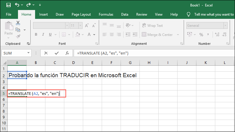
- Finally, add another comma and type the language code of the language in which you want the text to be translated, such as
enfor English and close the bracket.
- Hit Enter and you should now see that your text has been translated successfully.
Using the DETECTLANGUAGE function
The DETECTLANGUAGE function can help you find the code for the language used in a cell, making it easy to identify the language.
- Open a new Excel worksheet and paste some text in the language you wish to identify.

- Go to another cell and type
=DETECTLANGUAGE(.
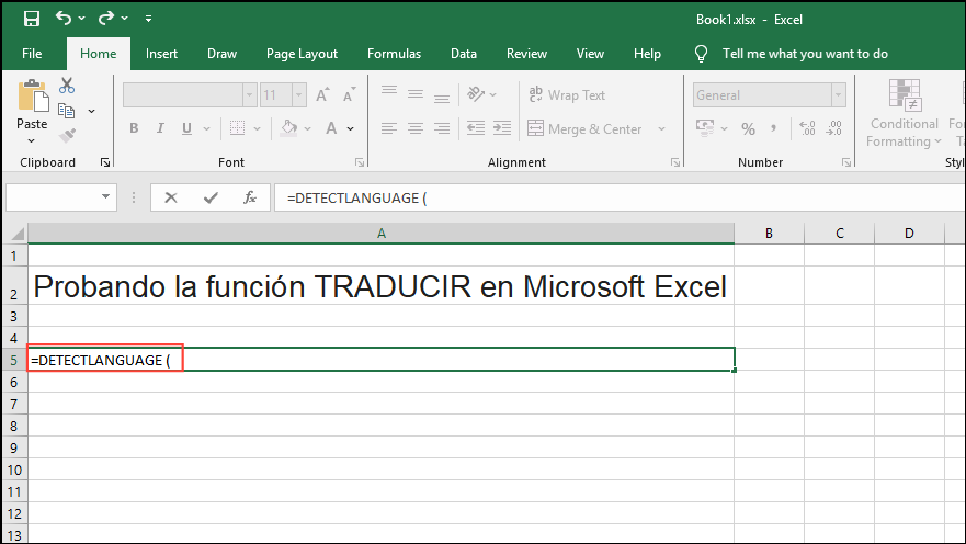
- Then add the address of the cell containing the text whose language you want to identify.
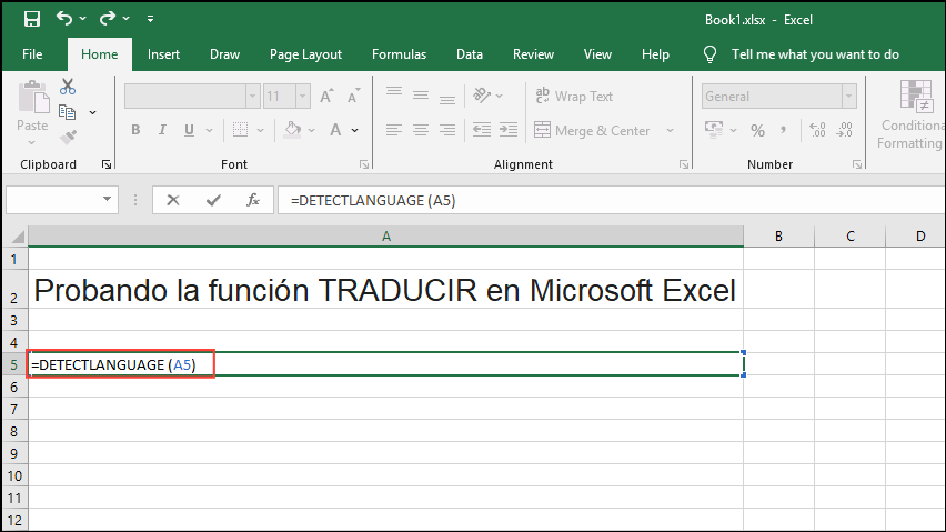
- When you press Enter, Excel should show you the code of the language used in the cell. In this case, you should see 'es' for Spanish.
Make translations dynamic
You can use other Excel tools, like adding dropdowns to make your translations dynamic and enhance the user experience.
- First, you need to create a list of the languages you want users to pick from. Click on the '+' button at the bottom to open a new Excel sheet.'
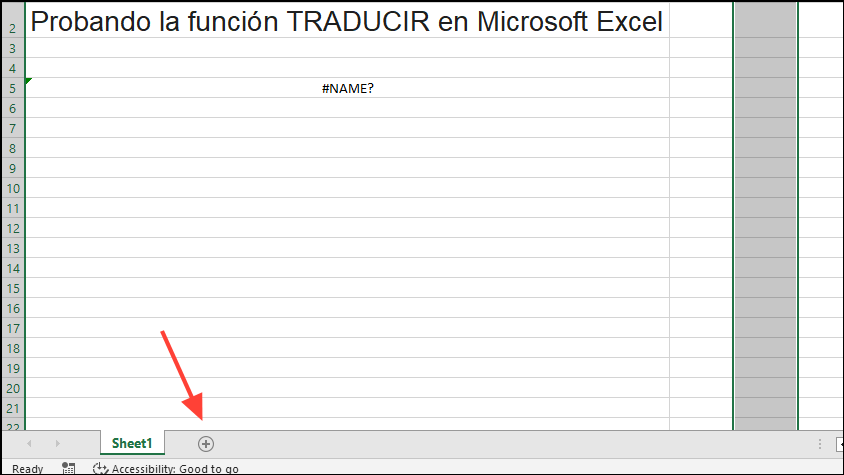
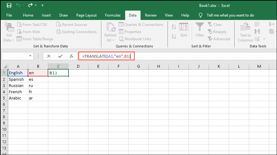
- When the new sheet opens, type the languages you want to add in Column A in different rows. Then fill Column B with their corresponding language codes.
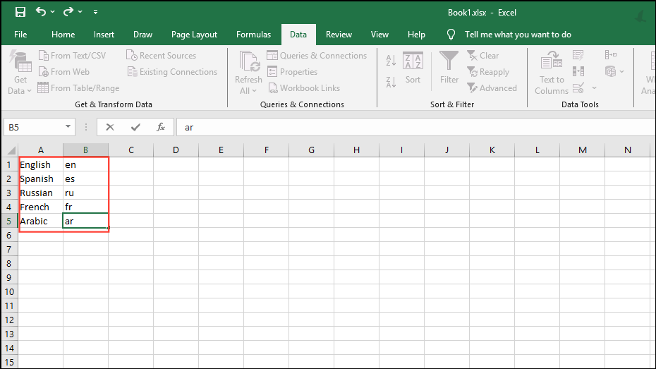
- Click on Cell C1, type
=TRANSLATE(A1,"en",B1)and press Enter. Then bring your cursor to the right edge of the cell and drag it down to fill the rest of the cells with the translations.
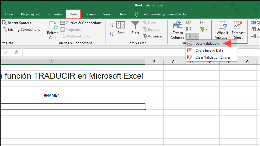
- Now, go back to Sheet 1 by clicking on it at the bottom left and select the cell where you want to create the dropdown. Then, go to the 'Data' tab at the top and then click on 'Data Validation'.
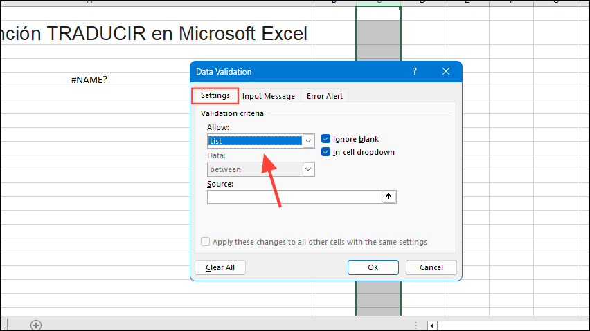
- In the Data Validation dialog box, select 'List' in the dropdown on the 'Settings' tab.
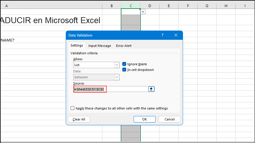
- In the Source field, select the cells containing the language translations in Sheet 2. Press Enter and a dropdown will be added in the cell you selected earlier, with the languages you added in Sheet 2.
- Depending on how you have entered the data in your worksheet, you can use or modify the following formula to link the TRANSLATE function with the dropdown:
=TRANSLATE(A3,"en",XLOOKUP($B$1,Sheet2!$C$1:$C$3,Sheet2!$B$1:$B$3).
Things to know
- The TRANSLATE and DETECTLANGUAGE functions have only been added recently to Excel, so they may not yet be available on your system.
- Due to the difference in the number of characters between different languages, they appear differently. To ensure uniformity and make sure your Excel worksheet has a clean appearance, you can adjust the fonts by changing their sizes, colors, etc., after using the translation function.
- If you get the 'Text too long' error, you need to reduce the characters in the cell and the cell size. Similarly, to fix 'Error in value', make sure the cell does not contain any non-text value and remove it if it does. The 'Invalid language' error appears if you have entered an incorrect or unsupported language code.
- For the TRANSLATE and DETECTLANGUAGE functions, you need to be connected to the internet, since they rely on Microsoft's Translation Services. Additionally, there is a limit to how many times you can use them. If you exceed your daily quota, you will see the 'Request Throttled' message and will have to wait till the quota resets.

