
The VLOOKUP function in Microsoft Excel is a powerful tool for searching data within a table organized vertically. Standing for “Vertical Lookup,” VLOOKUP searches for a specific value in the first column of a range and returns a corresponding value from a specified column to the right.
Imagine you have an inventory spreadsheet containing item names, purchase dates, quantities, and prices. Using VLOOKUP, you can swiftly retrieve the quantity and price of a particular item from this inventory, even if you’re working on a different worksheet.
While VLOOKUP might seem complex at first glance, it becomes straightforward once you grasp its functionality. This guide will walk you through how to effectively use the VLOOKUP function in Excel.
Understanding the VLOOKUP Function
Before diving into examples, it’s essential to comprehend the syntax and components of the VLOOKUP function.
The VLOOKUP function follows this syntax:
=VLOOKUP(lookup_value, table_array, col_index_num, [range_lookup])This function consists of four arguments:
- lookup_value: The value you want to find in the first column of the range. This value should be in the leftmost column of your data set.
- table_array: The range of cells where VLOOKUP will search and retrieve data. This range can be on the same worksheet, a different worksheet, or even in another workbook.
- col_index_num: The column number in the table_array from which to return the matching value.
- [range_lookup]: An optional argument that determines the type of match. Use
FALSEfor an exact match orTRUEfor an approximate match.
Using the VLOOKUP Function in Excel
Let’s explore how to implement the VLOOKUP function with practical examples.
Basic Example of VLOOKUP
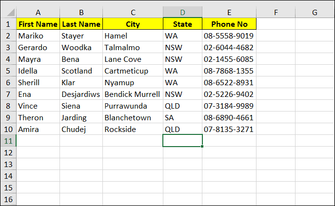
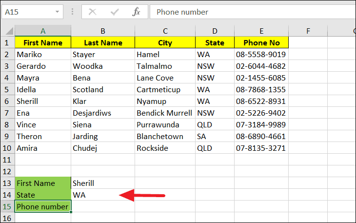
First, set up your data table that VLOOKUP will reference. Below is an example inventory list:
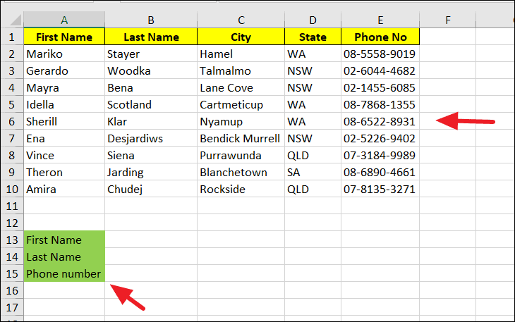
Next, create a separate area or table where you want to display the retrieved data from the main table.
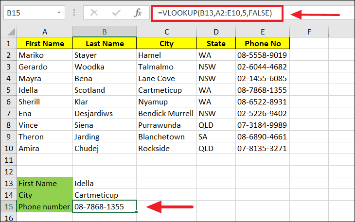
Suppose you want to find the phone number of “Ena” from the inventory. Place your cursor in the cell where you want the phone number to appear and enter the VLOOKUP formula. In this case, the formula would be:
=VLOOKUP(B13, A2:E10, 5, FALSE)Here’s what each argument represents:
B13is the cell containing the lookup value “Ena”.A2:E10is the range of the main table.5indicates the 5th column in the range, which contains the phone numbers.FALSEspecifies that we want an exact match.
You can select the table range directly with your mouse when entering the formula, which adds the range to your formula automatically.
It’s important to note that the lookup_value must be in the leftmost column of the specified range for VLOOKUP to work correctly. In this example, “Ena” should be in the first column of A2:E10.
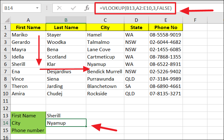
Direction of Lookup
The VLOOKUP function can only search for values in the first column and retrieve data from columns to the right. It does not look to the left of the lookup column.
Exact Match with VLOOKUP
When using VLOOKUP, you can specify whether you need an exact match or an approximate match using the [range_lookup] argument. Setting this argument to FALSE or 0 tells Excel to find an exact match.
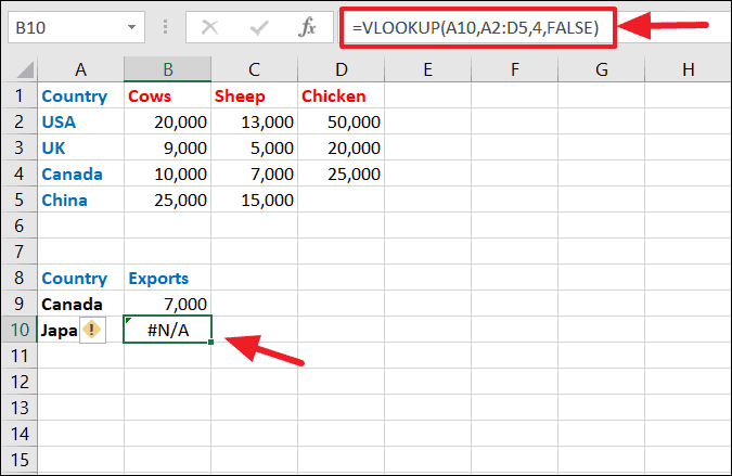
=VLOOKUP(A9, A2:D5, 3, FALSE)If the exact value is not found, VLOOKUP will return a #N/A error. For instance, if you’re searching for “Japan” in a list that doesn’t include it, the function will display an error.
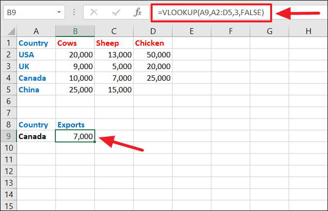
In this case, since “Japan” isn’t present in the lookup column, the function cannot find a match.
You can use either FALSE or 0 for an exact match; both are acceptable and function identically in Excel.
Approximate Match with VLOOKUP
Sometimes, you might need an approximate match rather than an exact one. To perform an approximate match, set the [range_lookup] argument to TRUE or omit it entirely, as TRUE is the default value.
=VLOOKUP(B10, A2:B7, 2, TRUE)For example, when assigning grades based on score ranges, an approximate match is suitable. If a student’s score isn’t an exact match in the table, VLOOKUP will find the next largest value that’s less than the lookup value.
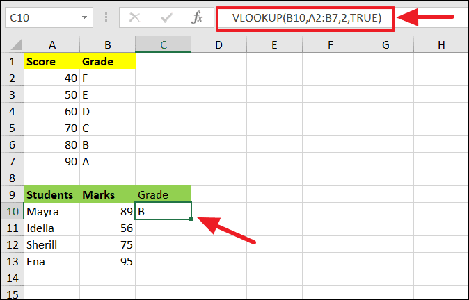
In this scenario, a score of 89 doesn’t have an exact match, so VLOOKUP returns the grade for the score 80.
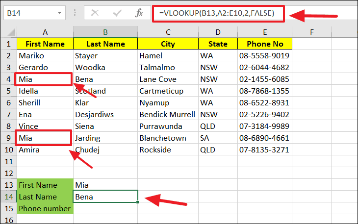
Handling Duplicate Values
When the lookup column contains duplicate values, VLOOKUP will return the first match it encounters. For instance, if you’re searching for “Mia” and there are multiple entries with that name, the function will retrieve data associated with the first “Mia” it finds.
Using Wildcards in VLOOKUP
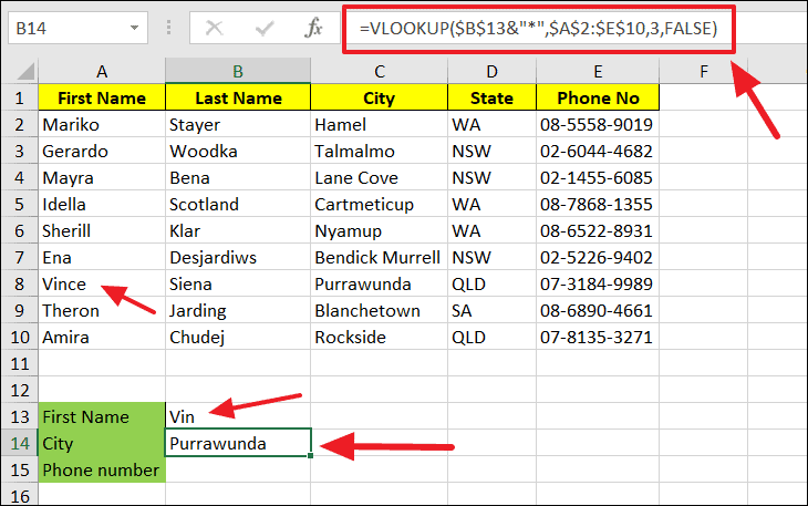
VLOOKUP supports the use of wildcard characters for partial matches. This is helpful when you only know part of the lookup value. To use wildcards, include an asterisk (*) in your lookup value. Concatenate the wildcard with your cell reference using an ampersand (&).
=VLOOKUP($B$13&"*", $A$2:$E$10, 3, FALSE)In this formula, if B13 contains “Vin”, the function will search for any value that starts with “Vin” and return the corresponding data.
Performing Multiple Lookups
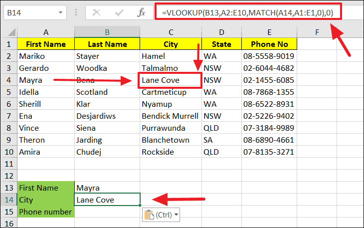
You can create dynamic lookups by combining VLOOKUP with other functions like MATCH. This allows you to search based on both row and column criteria.
=VLOOKUP(B13, A2:E10, MATCH(A14, A1:E1, 0), 0)In this example, VLOOKUP searches for the first name “Mayra” and uses the MATCH function to find the column number for “City”.
VLOOKUP from Another Sheet
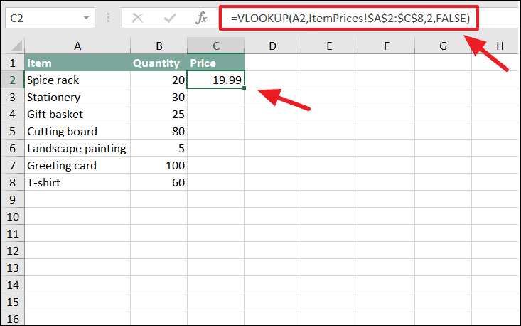
VLOOKUP is often used to retrieve data from a different worksheet within the same workbook. To reference another sheet, include the sheet name followed by an exclamation mark (!) before the range in your formula.
=VLOOKUP(A2, ItemPrices!$A$2:$C$8, 2, FALSE)Here, the function looks up the value in cell A2 on the current sheet and searches for it in the range $A$2:$C$8 on the ItemPrices sheet.
The lookup table on the ItemPrices sheet might look like this:
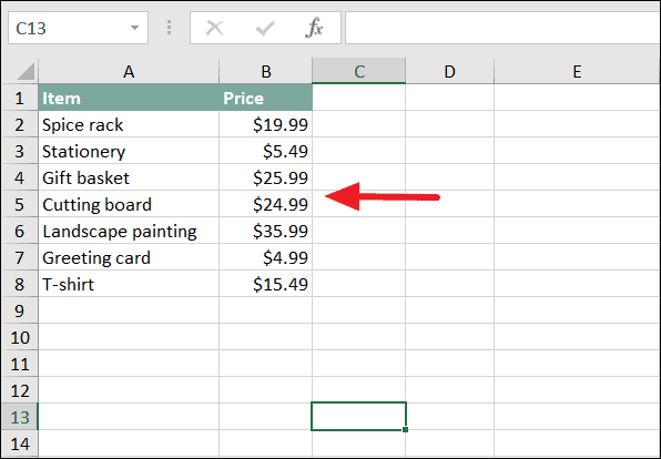
When you use the VLOOKUP formula on your current sheet, it fetches the corresponding prices from the ItemPrices sheet.
VLOOKUP from Another Workbook
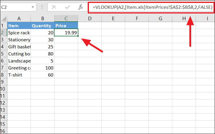
You can also use VLOOKUP to retrieve data from a different workbook. To do this, include the workbook name in square brackets followed by the sheet name and range.
=VLOOKUP(A2, [Item.xls]ItemPrices!$A$2:$B$8, 2, FALSE)When setting up the formula, it’s best to have both workbooks open. Navigate to the other workbook when selecting the table_array range to automatically include the correct path.
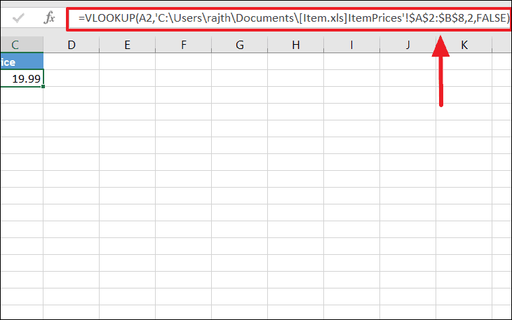
If the source workbook is closed, Excel will display the full file path in the formula, but the VLOOKUP will still work correctly.
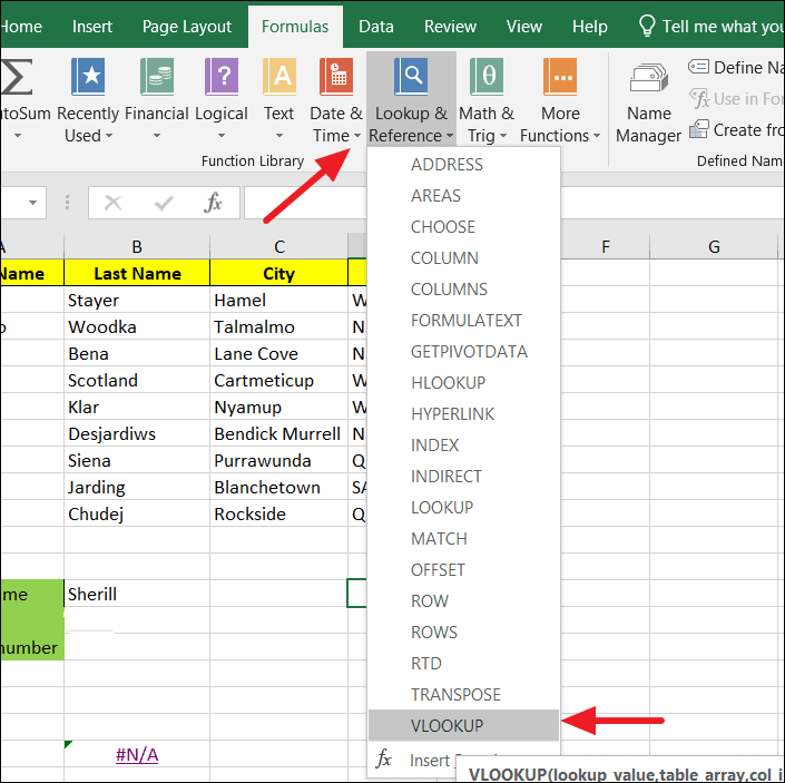
Accessing VLOOKUP from the Excel Ribbon
If you prefer using the interface rather than typing formulas, you can access VLOOKUP from the Excel Ribbon. Go to the Formulas tab, click on Lookup & Reference, and select VLOOKUP from the dropdown menu.
In the Function Arguments dialog box that appears, fill in each argument with the appropriate values and ranges. Click OK to apply the function.
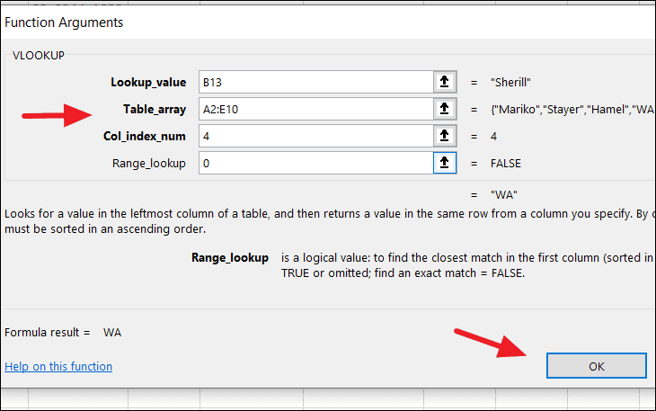
For example, searching for the first name “Sherill” in your table to find the corresponding state would look like this:
By understanding and utilizing the VLOOKUP function, you can efficiently search and manipulate data across your Excel worksheets and workbooks.


