Hidden rows and columns in Excel can lead to missing data in your spreadsheets, causing confusion or errors in your work. Thankfully, Excel provides several ways to unhide these rows and columns, ensuring you have full access to all your data.
Unhiding Rows in Excel
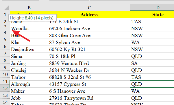
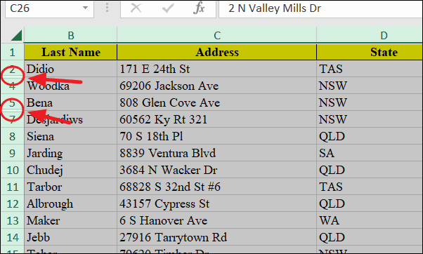
Identifying hidden rows in Excel is straightforward. If a row number is missing and there’s a double line between adjacent row numbers, it indicates that a row is hidden between them.
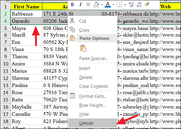
Select the rows above and below the hidden row by clicking on their row numbers. For example, if row 2 is hidden between rows 1 and 3, select rows 1 and 3.
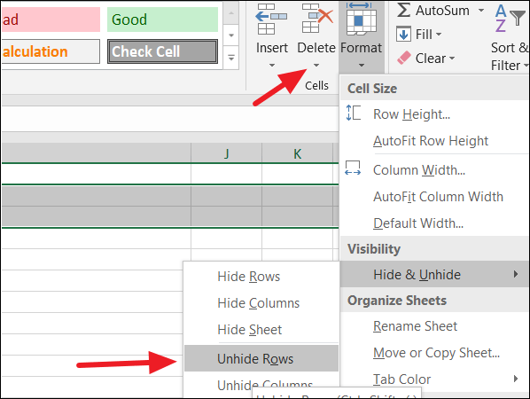
Right-click anywhere on the selected row numbers and choose Unhide from the context menu.
Unhiding Columns in Excel
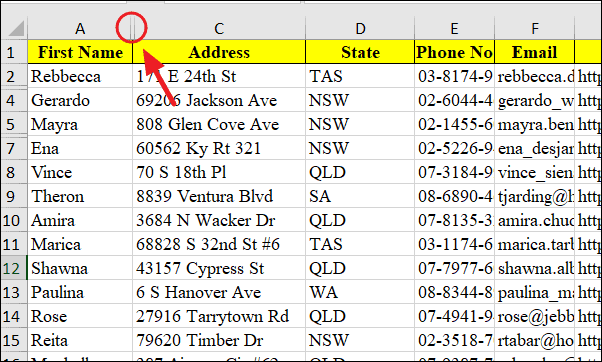
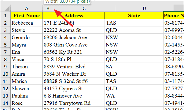
Hidden columns in Excel can also conceal important data. Similar to rows, hidden columns can be identified by missing column letters and a double line between column headers.
To unhide a hidden column using the right-click method:
Select the columns adjacent to the hidden column by clicking on their column letters. For example, if column B is hidden between columns A and C, select columns A and C.
Place your cursor on the boundary between the column headers of the columns adjacent to the hidden column. The cursor will change to a double-headed arrow.
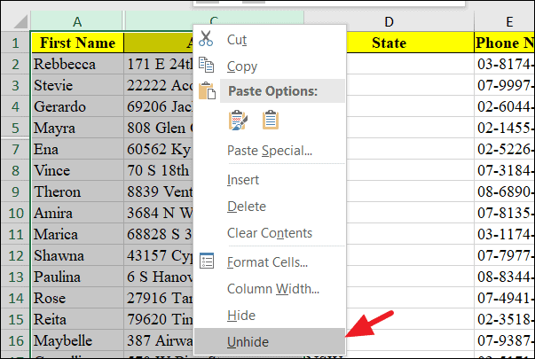
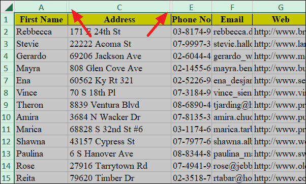
Right-click on any column header and choose Unhide from the context menu.
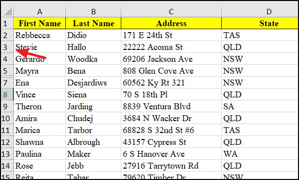
By following these methods, you can easily unhide any rows or columns in your Excel worksheet, ensuring all your data is visible for analysis and presentation.