
Conditional formatting rules in Excel can stop working when formulas are misconfigured, ranges are set incorrectly, or cell data types don't match rule requirements. This leads to missing highlights, colors not appearing, or inconsistent formatting across your spreadsheets. Addressing these issues requires a methodical check of rule formulas, cell formats, and the order of applied rules.
Check Formula Logic and Cell References
Incorrect formula syntax or improper use of absolute and relative cell references disrupts conditional formatting. Excel applies the formula to each cell in the specified range, so references must align with how the rule is meant to work. For example, using =$A$2="TEXT" will lock the rule to cell A2, but =A2="TEXT" will adjust for each row.
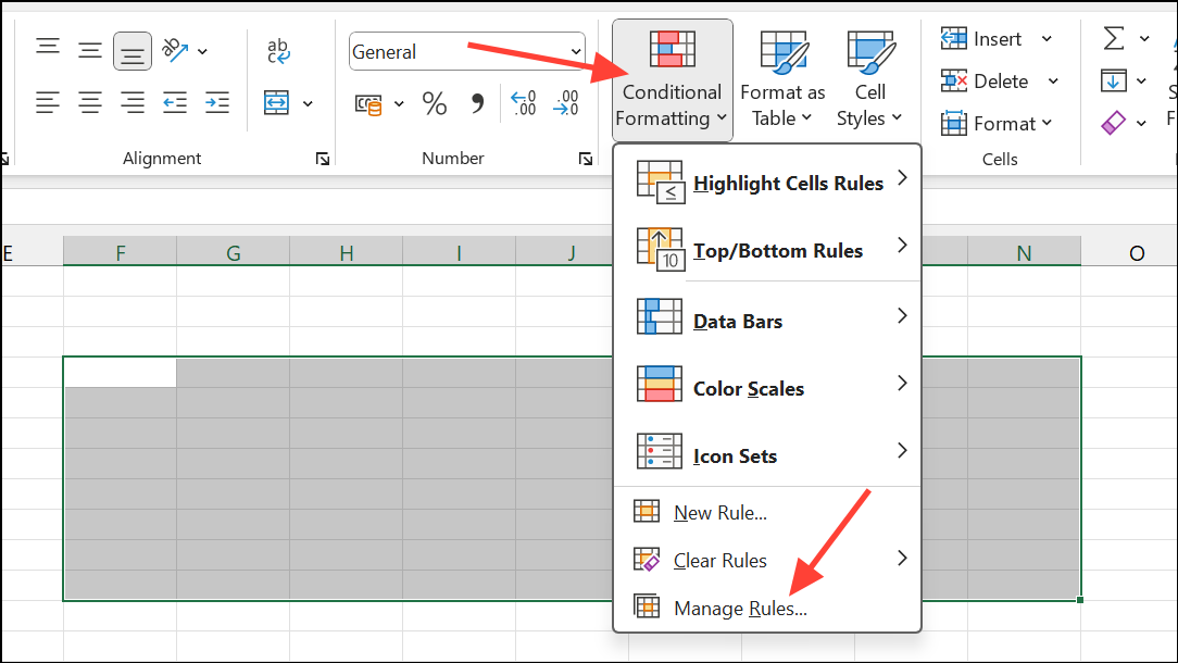
Step 1: Open the Conditional Formatting Rules Manager by selecting your formatted range, then navigating to the Home tab and clicking "Conditional Formatting" > "Manage Rules".
Step 2: Select the rule and examine the formula. Check if you are using the correct reference style:
- Absolute references (e.g.,
=$A$2) keep both row and column fixed. - Mixed references (e.g.,
=$A2) fix the column but allow the row to change. - Relative references (e.g.,
=A2) adjust both row and column as the rule is applied across the range.
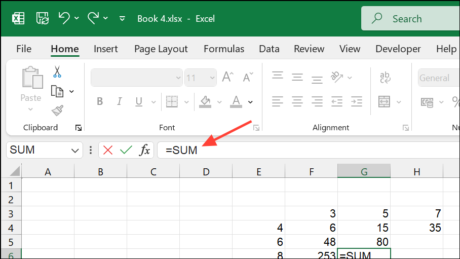
Step 3: Ensure the formula starts with an equals sign (=). Omitting this prevents Excel from evaluating the formula.
Step 4: For rules using formulas, confirm the formula returns only TRUE or FALSE. If it returns other values or errors, the rule will not apply.
Verify the Range Applied to the Rule
If conditional formatting only works for part of your data, the "Applies to" range may be incomplete or misaligned. Excel can also behave unexpectedly if you copy rules without updating the "Applies to" range or formula references.
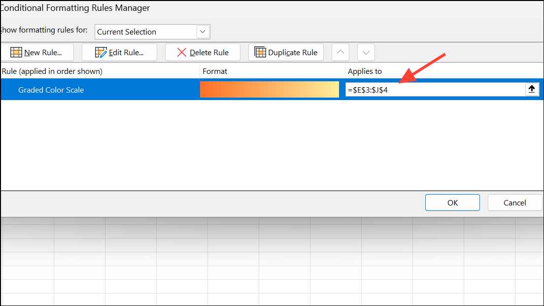
Step 1: In the Conditional Formatting Rules Manager, check the "Applies to" field for each rule. The range should match the intended cells (e.g., =$A$2:$A$100 for a single column, or =$A$2:$H$100 for multiple columns).
Step 2: If you need the rule to apply to several non-contiguous ranges, list them separated by commas (e.g., =$Z$4:$Z$16,$Z$19:$Z$31).
Step 3: Adjust the formula so that it works as if it is being applied to the first cell of the "Applies to" range. For example, if your range starts at row 2, write the formula as if for that row (e.g., =A2="TEXT").
Check Cell Data Types and Formatting
Conditional formatting rules that rely on numbers or percentages will not work correctly if the underlying cell format is set to text or another incompatible type.
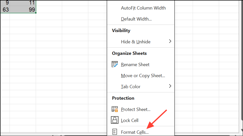
Step 1: Select the cells you want to check, then go to the Home tab and click "Format" > "Format Cells".
Step 2: In the Format Cells dialog, check the "Number" tab. Ensure the appropriate format (Number, Percentage, Date, etc.) is selected for your data.
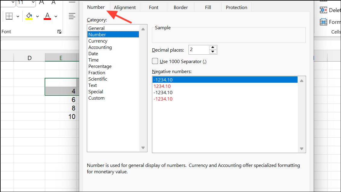
Step 3: If the format is incorrect (e.g., text instead of number), change it to the correct type and reapply or refresh your conditional formatting rules.
Cells formatted as text may not evaluate as numbers in rules, leading to missing or incorrect formatting. Reformatting to the correct type allows rules to work as intended.
Resolve Rule Conflicts and Rule Order
When multiple conditional formatting rules overlap, Excel applies them in order from top to bottom. If two rules set the same property (like background color) for the same cell, the higher rule takes precedence.
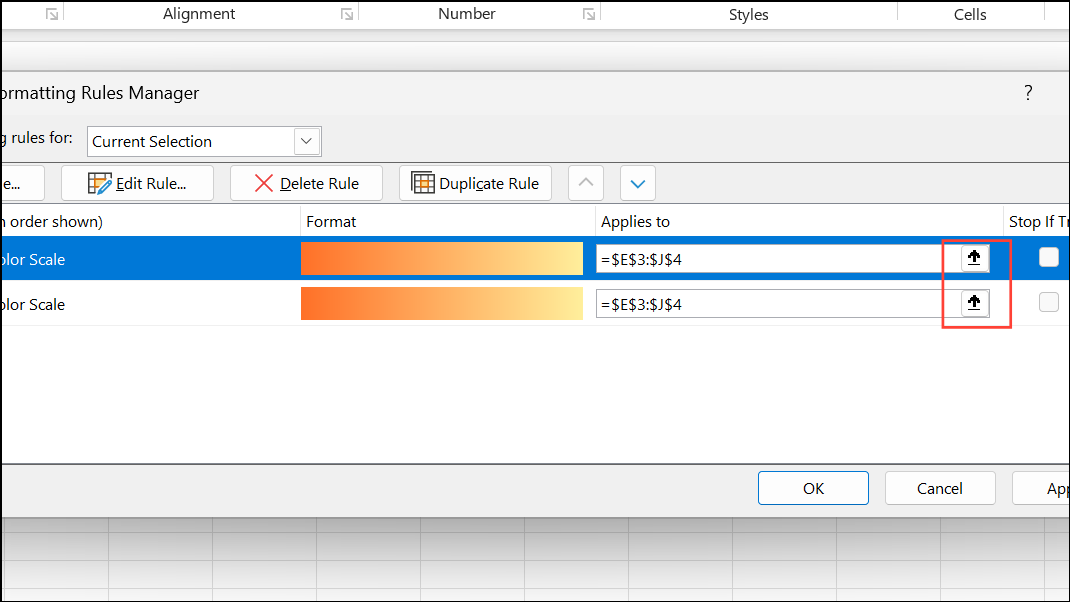
Step 1: Open the Conditional Formatting Rules Manager and review the order of your rules.
Step 2: Use the "Move Up" and "Move Down" buttons to change rule priority. Place more specific or higher-priority rules above more general ones.
Step 3: If two rules conflict, ensure only one sets a particular property for a given cell or adjust the ranges so they do not overlap unnecessarily.
For example, if one rule sets the background color for values greater than 95% and another for values less than 95%, overlapping ranges can cause only the top rule to be visible.
Address File Corruption or Compatibility Issues
Corrupted Excel files or version incompatibilities can cause conditional formatting to stop working or behave inconsistently, especially when opening files created in newer Excel versions with older software.
Step 1: Save your workbook and close Excel.
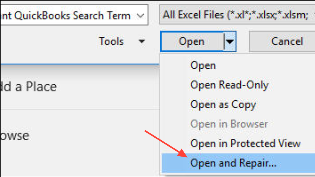
Step 2: Reopen Excel, go to File > Open, select your file, and choose "Open and Repair" from the dropdown next to the Open button.
Step 3: If the file repairs successfully, check if conditional formatting now works as expected. For persistent issues, try recreating the rules in a new worksheet.
Step 4: If you are using features available only in newer Excel versions, consider saving the workbook in a compatible format or updating your software.
Tips for Creating Effective Conditional Formatting Rules
- Always write formulas as if for the first cell in the "Applies to" range.
- Use absolute references only when you want a fixed cell across all formatted cells.
- Test rules on a small sample before applying to large ranges.
- Regularly review the order and overlap of your rules to avoid conflicts.
- For complex logic, use "Use a formula to determine which cells to format" and test the formula in a worksheet cell first.
By systematically reviewing formulas, ranges, cell formats, and rule order, you can restore conditional formatting functionality and achieve consistent, visually clear results in your Excel spreadsheets.
Once you align cell references, ranges, and data types, conditional formatting will apply rules reliably and accurately highlight your data.