
Excel formulas can display errors such as #DIV/0! and #VALUE! when calculations encounter invalid data or unexpected input. These errors can disrupt data analysis, cascade into other formulas, and make reports difficult to interpret. Addressing them promptly streamlines your workflow and ensures your results remain accurate for further processing.
Fixing #DIV/0! Errors in Excel
The #DIV/0! error appears when a formula attempts to divide by zero or an empty cell. For example, =A1/B1 returns #DIV/0! if B1 contains zero or is blank. This error can also occur in aggregate functions like AVERAGE or AVERAGEIF if the denominator is missing or all values are non-numeric.
Step 1: Identify the cell causing the error by checking the formula and the referenced denominator. If the denominator cell is blank or contains zero, update it with a valid value if appropriate for your data.
Step 2: If you expect blank or zero denominators as part of your workflow, wrap your formula in an error-handling function to suppress the error and display a more useful result.
Method 1: Using IFERROR to Handle #DIV/0! and Other Errors
The IFERROR function detects any error in a formula and lets you specify a fallback value. This approach is concise and works for a wide range of errors, not just #DIV/0!.
Step 1: Replace your formula with an IFERROR wrapper. For example, to show zero instead of #DIV/0!:
=IFERROR(A1/B1, 0)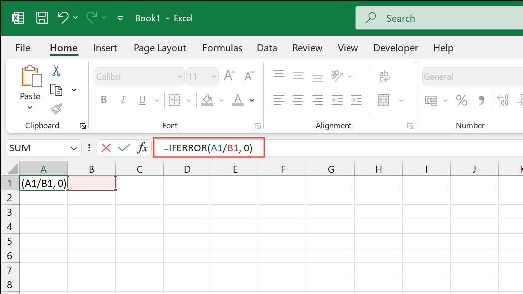
This formula returns the result of A1/B1 unless an error occurs, in which case it returns 0. You can substitute 0 with an empty string "" or a custom message like "Input Needed".
Step 2: Drag the formula down or across your worksheet to apply it to additional cells as needed.
IFERROR suppresses all error types, including #N/A, #VALUE!, #REF!, and others. Ensure your formulas are working as intended before applying this method, as it may hide underlying issues.Method 2: Using IF to Check the Denominator
For division formulas, you can prevent #DIV/0! errors by checking if the denominator is valid before performing the calculation.
Step 1: Use an IF statement to test if the denominator is not zero or blank. For example:
=IF(B1, A1/B1, 0)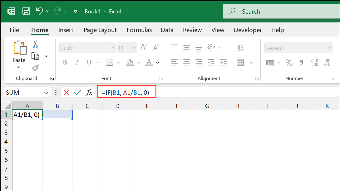
This formula checks if B1 contains a non-zero, non-blank value. If so, it calculates A1/B1; otherwise, it returns 0. You can also return an empty string or a custom message as needed.
Step 2: Copy the formula to other cells to apply the same logic throughout your worksheet.
This approach is especially useful for simple division operations where you want to avoid using IFERROR and only target cases where the denominator is zero or blank.
Method 3: Using ERROR.TYPE for Advanced Error Handling
The ERROR.TYPE function returns a number corresponding to the type of error in a formula. For example, #DIV/0! returns 2 and #VALUE! returns 3. This allows you to handle specific errors differently.
Step 1: Use ERROR.TYPE within an IF statement to detect #DIV/0! and return a specific value:
=IF(ERROR.TYPE(A1/B1)=2, 0, A1/B1)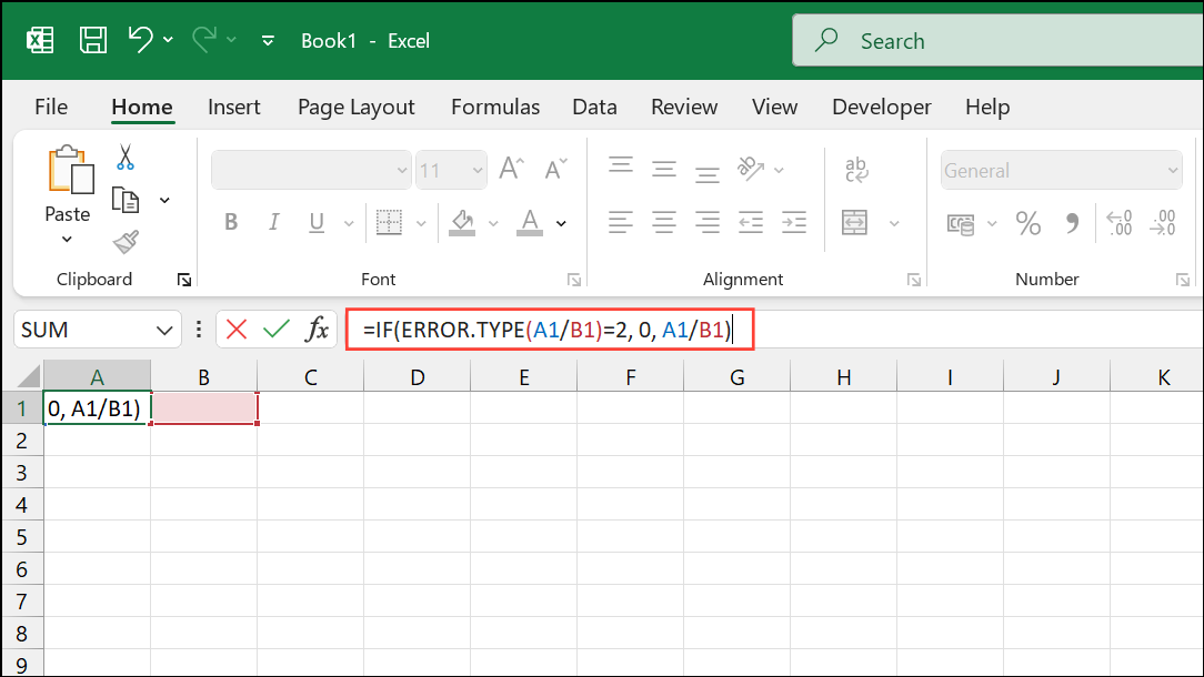
This formula checks if A1/B1 returns a #DIV/0! error and outputs 0 if true, otherwise it returns the calculation result. Adjust the number in ERROR.TYPE() to target other error types as needed.
This method is best for advanced users who need granular control over error responses in complex formulas.
Fixing #VALUE! and Other Common Excel Errors
The #VALUE! error typically occurs when a formula uses the wrong data type, such as trying to perform arithmetic on text. To resolve this, check all referenced cells for unexpected text, blanks, or non-numeric data.
Step 1: Review formula arguments and ensure all referenced cells contain valid numeric values. If a cell contains text or a special character, correct it to a number if possible.
Step 2: Use IFERROR to catch and manage #VALUE! errors, especially in larger datasets where manual correction is impractical:
=IFERROR(A1+B1, 0)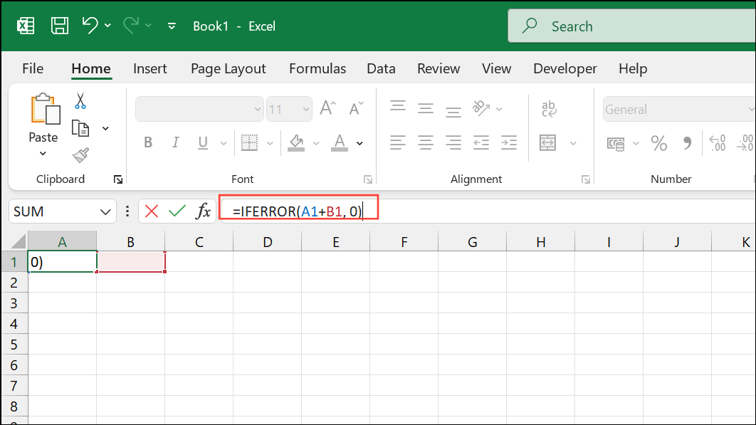
This formula adds A1 and B1. If either cell contains text or an invalid value, the result is 0 instead of an error.
For more targeted error handling, combine IF with ISNUMBER or ISTEXT to check data types before performing calculations.
Handling Errors in Array and Aggregate Formulas
Complex formulas, such as those using AVERAGE or arrays, may encounter errors in one or more terms. To avoid a single error disrupting the entire result, wrap each term with IFERROR and use functions like COUNT to calculate averages only on valid results.
Step 1: For a formula like:
=AVERAGE((F2/SUM(F2:I2)), (K2/SUM(J2:M2)), (P2/SUM(N2:Q2)), (U2/SUM(R2:U2)))wrap each term with IFERROR and calculate the sum and count of valid terms:
=SUM(IFERROR(F2/SUM(F2:I2),0), IFERROR(K2/SUM(J2:M2),0), IFERROR(P2/SUM(N2:Q2),0), IFERROR(U2/SUM(R2:U2),0))
    /COUNT(IFERROR(F2/SUM(F2:I2),""), IFERROR(K2/SUM(J2:M2),""), IFERROR(P2/SUM(N2:Q2),""), IFERROR(U2/SUM(R2:U2),""))
This method ensures that only valid results are included in the average, preventing errors from skewing calculations or causing the entire formula to fail.
Resolving Excel errors like #VALUE! and #DIV/0! keeps your spreadsheets reliable and calculations on track. Adopting these error-handling techniques will make it easier to maintain and update your work in the future.