The Excel MATCH function searches for a specified value in a range of cells and returns the relative position of that value within the range. Unlike the VLOOKUP function, which retrieves a value, the MATCH function locates the position of a value, which is particularly useful in various lookup scenarios.
The MATCH function scans a range of cells or an array for a specified value and returns the position of its first occurrence. When combined with the INDEX function, it can be used to retrieve corresponding values, similar to how VLOOKUP operates. This guide will demonstrate how to utilize the MATCH function to determine the position of a lookup value in Excel.
Excel MATCH function
The MATCH function is a built-in feature in Excel that is primarily used to find the relative position of a specified value within a column or a row.
Syntax of the MATCH function:
=MATCH(lookup_value, lookup_array, [match_type])Where:
lookup_value – The value you want to find in the range. It can be a number, text, logical value, or a cell reference containing the value.
lookup_array – The range of cells or array where you want to search for the lookup_value. It should be a single row or column.
match_type – An optional argument that specifies how the function matches the lookup_value with values in the lookup_array. The default value is 1. It can be set to 1, 0, or -1.
- 0 – Finds the first value exactly equal to
lookup_value. If no match is found, it returns an error. - 1 – Finds the largest value less than or equal to
lookup_value. Thelookup_arraymust be sorted in ascending order. - -1 – Finds the smallest value greater than or equal to
lookup_value. Thelookup_arraymust be sorted in descending order.
Find position of an exact match
Suppose you have the following dataset and need to find the position of a specific city in the list.
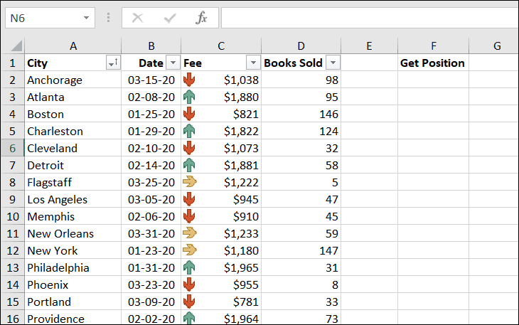
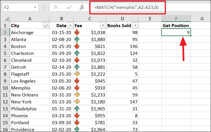
To locate the position of the city “Memphis” within the range A2:A23, you can use the following formula:
=MATCH("memphis", A2:A23, 0)The third argument is set to 0 to find an exact match. Notice that even though “memphis” is entered in lowercase in the formula, and “Memphis” in the dataset has an uppercase “M”, the function still finds the match because the MATCH function is not case-sensitive.
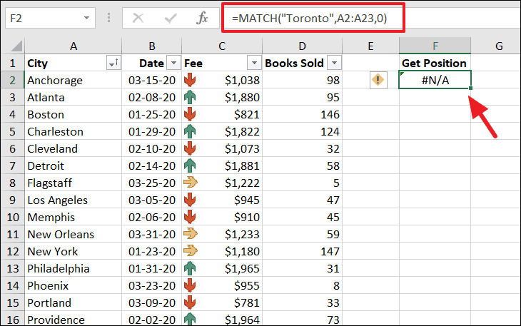
Note: If the lookup_value is not found within the specified lookup_array, or if the range is incorrect, the function will return a #N/A error.
Alternatively, you can use a cell reference for the lookup_value instead of typing the value directly. For example, the following formula uses the value in cell F2 to find its position in the range:
=MATCH(F2, A2:A23, 0)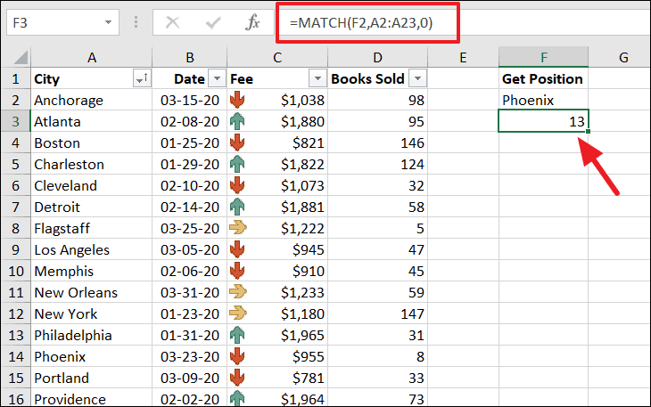
Find position of an approximate match
There are situations where you might need to find an approximate match rather than an exact one. The match_type argument controls how the MATCH function performs this search:
- 1 – Finds the largest value less than or equal to
lookup_value. Thelookup_arraymust be sorted in ascending order. - -1 – Finds the smallest value greater than or equal to
lookup_value. Thelookup_arraymust be sorted in descending order.
Next smallest match
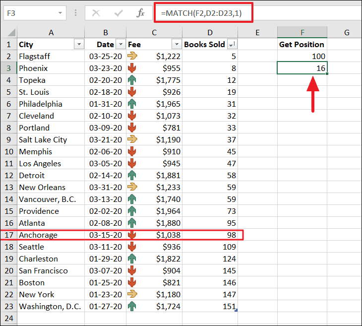
When the match_type is set to 1, and an exact match is not found, the MATCH function returns the position of the largest value that is less than or equal to the lookup_value. This requires the lookup_array to be sorted in ascending order.
For instance, suppose you have a range of numbers sorted in ascending order, and you want to find the position of a value that is closest to, but not exceeding, a specified number. Using match_type of 1, the formula would look like:
=MATCH(F2, D2:D23, 1)If the exact value in F2 is not found, the function returns the position of the next smallest value.
Next largest match
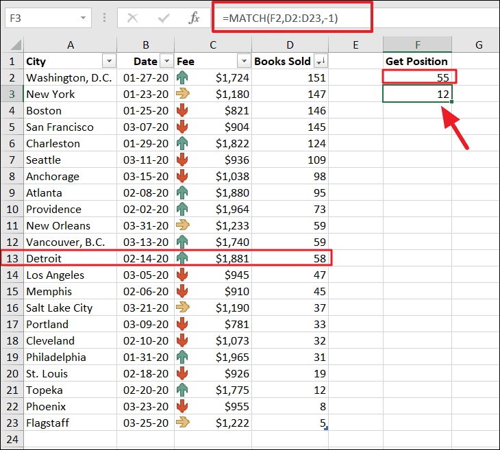
When the match_type is set to -1, the MATCH function returns the position of the smallest value that is greater than or equal to the lookup_value. In this case, the lookup_array must be sorted in descending order.
=MATCH(F2, D2:D23, -1)Assuming the values in D2:D23 are sorted in descending order, if an exact match is not found, the function returns the position of the next largest value.
Wildcard match
The MATCH function supports the use of wildcard characters when performing text searches, but only when match_type is set to 0. The two wildcard characters are:
- Question mark (?) – Matches any single character.
- Asterisk (*) – Matches any number of characters.
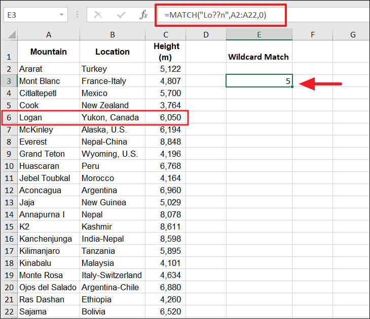
For instance, to find a city name that starts with “Lo”, followed by any two characters, and ends with “n”, you can use:
=MATCH("Lo??n", A2:A22, 0)This formula will match “London” in the list, as the two question marks “??” represent any two characters.
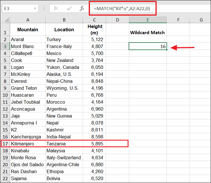
Similarly, you can use the asterisk (*) to match any number of characters. For example, to find a word that starts with “Kil”, has any number of characters in between, and ends with “o”, use:
=MATCH("Kil*o", A2:A22, 0)This formula will match “Kilimanjaro” in the list, and the function returns its position.
INDEX and MATCH
The MATCH function is often used in conjunction with the INDEX function to perform more powerful and flexible lookups in Excel. While VLOOKUP is commonly used for vertical lookups, combining INDEX and MATCH offers several advantages, such as the ability to perform lookups in any direction and improved performance.
The INDEX function returns a value from a range or array based on specified row and column numbers.
Syntax of the INDEX function:
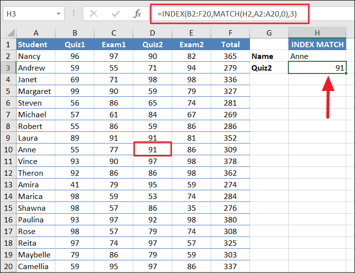
=INDEX(array, row_num, [column_num])For example, suppose you have a dataset of students’ scores, and you want to retrieve the score of a specific student in “Quiz2”. You can use the combined INDEX and MATCH functions as follows:
=INDEX(B2:F20, MATCH(H2, A2:A20, 0), 3)In this formula:
MATCH(H2, A2:A20, 0)finds the row number where the student’s name (in cellH2) appears in the rangeA2:A20.- The
INDEXfunction then uses this row number along with the specified column number (3 for “Quiz2”) to retrieve the desired score from the rangeB2:F20.
Two-way lookup with INDEX and MATCH
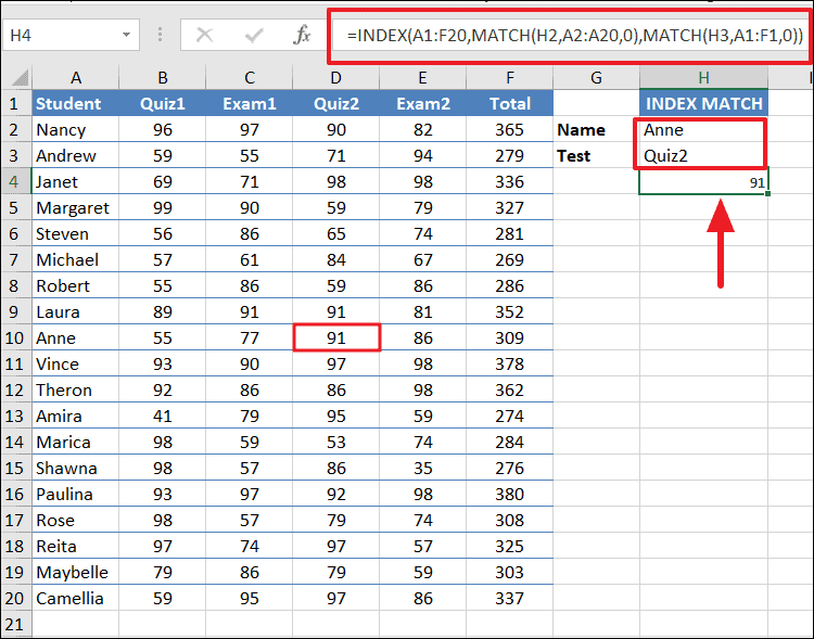
You can extend this approach to perform a two-way lookup by using two MATCH functions: one to find the row and another to find the column. This allows you to dynamically specify both the row and column in the INDEX function.
=INDEX(B1:F20, MATCH(H2, A2:A20, 0), MATCH(H3, B1:F1, 0))In this formula:
MATCH(H2, A2:A20, 0)finds the row number for the student name inH2.MATCH(H3, B1:F1, 0)finds the column number for the quiz name inH3.- The
INDEXfunction then retrieves the value at the intersection of that row and column in the rangeB1:F20.
By mastering the MATCH function and its combination with INDEX, you can perform more versatile and efficient lookups in Excel, enhancing your data analysis capabilities.


