
Subtracting time from another time is helpful if you want to find the time difference between two times. For example, if you want to find the time it took to complete a task, you can input both the start and end times of the task and subtract them to find the total elapsed time.
Since Excel stores dates and times as numbers, you can easily subtract using simple arithmetic formulas, TIME function, TEXT function, or TIMEVALUE function to calculate the time difference or elapsed time and more. In this article, we will see several methods to subtract time and calculate the difference between dates and times in Excel.
Calculate Time Difference Between Two Times
More than often, we need to calculate the time difference between two given times to find the elapsed time. You can calculate the time between two times or two cells with a simple subtraction.
The easiest way to find the time difference is by subtracting the Start time from the End Time:
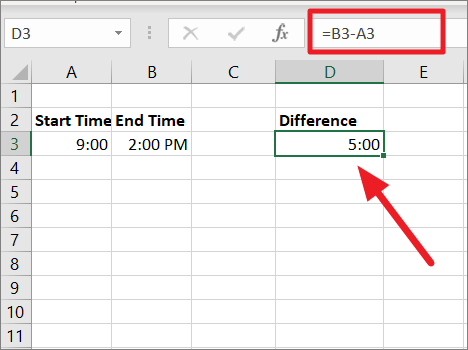
=End Time - Start TimeFor example, to subtract time in A3 from time in B3, we can use the below formula:
=B3-A3Where A3 is Start time and B3 is End Time. As you can see, there are 5 hours of difference between A3 and B3.
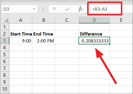
However, if the format of the result cell is set to General, you would get the results in fractions/decimals. It is because the time values are represented as fractions of a number in Excel.
In the Excel date system, time is stored like this:
In Excel’s internal system:
- 00:00:00 AM is stored as 0.0
- 06:00 AM is saved as 0.25
- 12:00 PM is stored as 0.5
- 18:00 PM is saved as 0.75
- 23:59:59 is stored as 0.99999
When you enter date and time into a cell, they will be stored as a serial number consisting of an integer and a decimal number. While the integer represents day/date, the number after the decimal point represents time. For instance, when you type ‘August 15, 2001, 6:00:00 AM’ in an Excel cell, it will be stored as ‘37118.25’.
So, the 5 hours will be displayed as ‘0.208333333’ as shown below.
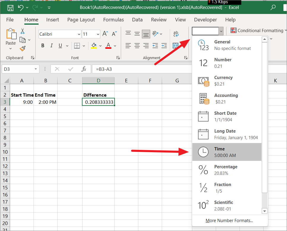
To display the decimals in Time, select the output cell. Then, click the ‘Number Format’ drop-down menu from the ‘Number’ group and select the ‘Time’ option.
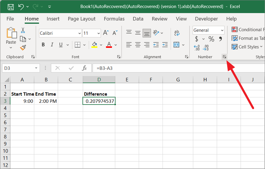
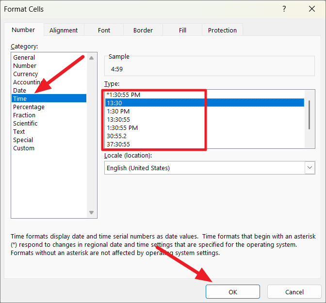
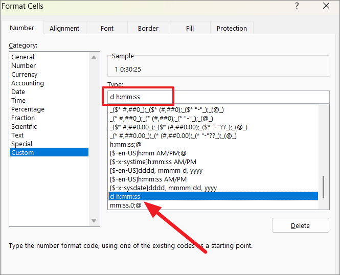
To apply the custom time format, click the arrow button (Number Format) at the corner of the Number group on the ribbon or press Ctrl+1 to open the Format Cells dialog box.
Under the Number tab, go to the ‘Time’ tab and choose one of the time formats and click ‘OK’.
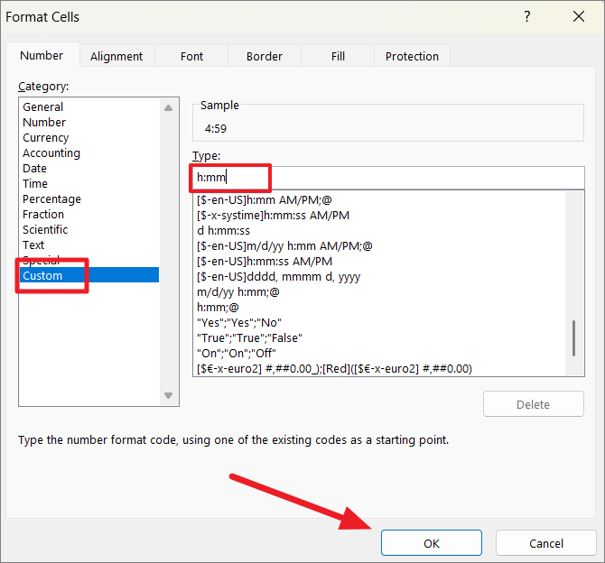
Or, you can go to the ‘Custom’ tab and type one of the following codes and click ‘OK’ to apply the respective time formatting:
| Time code | Use |
|---|---|
| h | To display time difference in hours. E.g. 5 |
| h:mm | To display time difference in hours and minutes. E.g. 5:30 |
| h:mm:ss | To display time differences in hours, minutes, and seconds. E.g. 5:30:10 |
| d h:mm:ss | To display time differences in days, hours, minutes, and seconds. E.g. 2 5:30:10 |
If the output is ##### error, it means either the output cell is not wide enough or the result is a negative number. If the result is negative, we will see how to handle the negative times in Excel in one of the following sections.
Count Hours, Minutes, or Seconds Between Two Times
Sometimes, we only want to calculate the time difference in individual time units (hours, minutes, or seconds). When you subtract times, Excel will always return decimal numbers. In the resulting value, every whole number represents a day and decimal numbers can be converted to hours, minutes, or seconds. To do that, use the following formulas:
Find Hours Between Two Times
To calculate the time difference between two times in hours, use this formula:
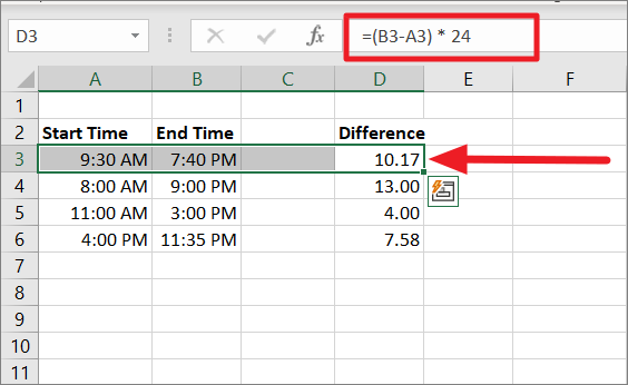
=(End time - Start time) * 24Example:
=(B3-A3) * 24Here the starting time is A3 and the ending time is B3. You can subtract B3-A3 to calculate the difference between the two times, then multiply it by 24 (which is the number of hours in a day). This gives us 10.17 as the result.
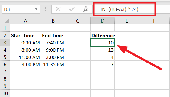
You can use the INT function to get the number of complete hours:
=INT((B3-A3) * 24)The INT function rounds up the result to give whole numbers.
Find Total Minutes Between Two Times
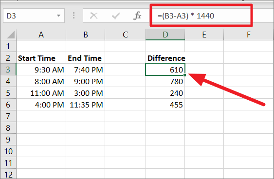
To calculate the time difference between two times in minutes, use this formula:
=(End time - Start time) * 1440or
=(End time -Start time ) * 24 * 60Example:
=(B3-A3) * 1440Where the starting time is A3 and the ending time is B3. You can use simple subtraction B3-A3 to find the difference between the two times, and then multiply it by 1440 which is the number of minutes in a day. The final output will be 610 which is the total minutes between A3 and B3.
Find Total Seconds Between Two Times
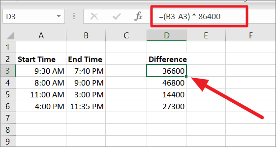
Use this formula to get the difference between two times in seconds:
=(End time - Start time) * 86400or
=(End time - Start time) * 24 * 60 * 60Example:
=(B3-A3) * 86400Where the starting time is A3 and the ending time is B3. You can use simple subtraction B3-A3 to find the difference between the two times, and then multiply it by 86400 which is the number of seconds in a day. The final output will be 36600, which is the total number of seconds between A3 and B3.
Calculate Elapsed Time from a Starting Time till Now using the Now () function
When you use the NOW function in Excel, it will display the current date and time from your Computer. If you want to find the elapsed time from a start time till now, i.e., current time, you can use the Now() function instead of the end time in the formula.
Here’s a formula that you can use to find the elapsed time:
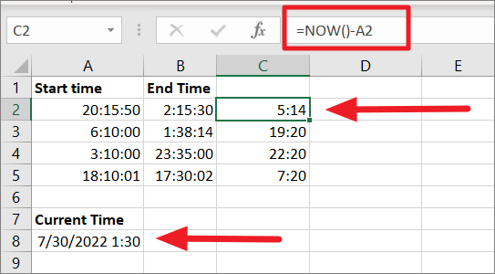
=Now-Start timeIn the below example, the start time is in column A. To calculate the elapsed time from the given start time till now, you can use the formula:
=NOW()-A1The resulting value for time elapsed till now is returned in column B. In case your starting times only have time units without dates, the formula may return the wrong results as shown below. It’s because Excel will consider the date as 1st January 1990 by default.
To fix this, you can either add the date portion to the starting time or use INT() function which will trim the day value returned by the NOW() function.
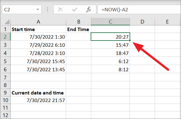
First, enter starting date and time in a cell(s), then, enter the same formula. Make sure to apply the appropriate time format to column C (result column), h:mm.
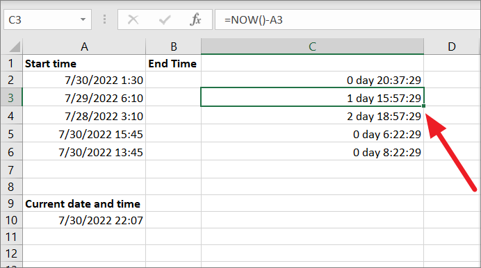
If the elapsed time exceeds 24 hours, you need to apply the time format to display days as well as time in the result. You can use any of the following formats to include days:
| Format | Example |
| d h:mm:ss | 1 15:57:29 |
| d “day” h:mm:ss | 1 day 15:57:29 |
| d “day,” h “hours,” m “minutes, and” s “seconds” | 1 day 15 hours 57 minutes and 29 seconds |
In the below example, we have applied the d "day" h:mm:ss format to the C column. As you can see, the elapsed time from the starting time (7/29/2022) till now is 1 day 15 hours, 57 minutes, and 29 seconds.
Calculate Time Difference Between Specified Times
You can directly calculate the time difference between two given times using the TIMEVALUE() function. With the TIMEVALUE function, you don’t need to enter the start and end times in two different cells, you can pass the values directly to the formula.
The Syntax:
=TIMEVALUE("Start Time") - TIMEVALUE("End Time")For example, to calculate the time difference between 6:10 and 3:00, use the below formula:
=TIMEVALUE("6:10 PM")-TIMEVALUE("3:00 PM")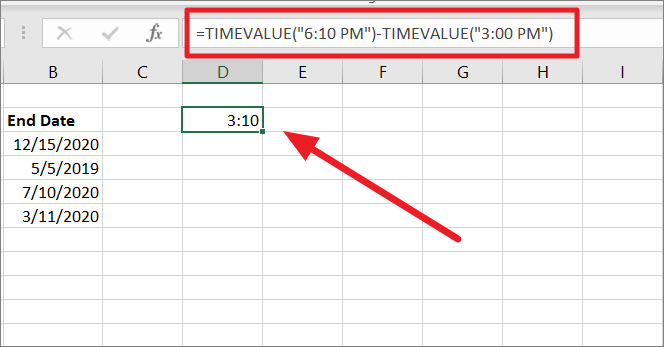
Calculate the Difference in Only One Time Unit
You can use HOUR(), MINUTE(), and SECOND() functions to calculate the time difference between two times in only one unit while ignoring the others.
To calculate the time difference in hours while ignoring minutes and seconds, use this sample formula:
=HOUR(A2-B2)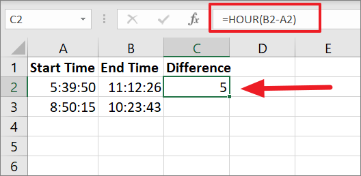
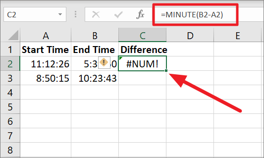
To calculate the time difference in minutes while ignoring minutes and seconds, use this sample formula:
=MINUTE(A2-B2)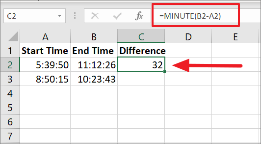
To calculate the time difference in seconds while ignoring minutes and seconds, use this sample formula:
=SECOND(A2-B2)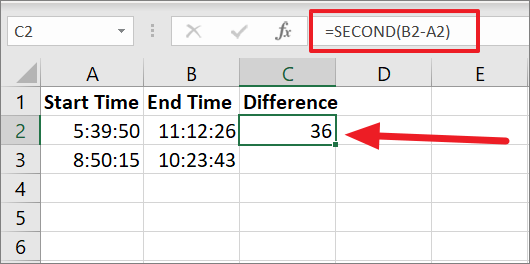
However, if the end time is less than the start time, the result will be a negative number. Thus, you will get a NUM! error as a result.
Make sure the result of the HOUR() function doesn’t exit 24 hours and the result of MINUTE() and SECOND() functions don’t exit 60 minutes and 60 seconds respectively.
Subtract Time to Find Time Difference using the Text Function
If you don’t want to change the format of the cells, you can use the TEXT function to calculate and output the time difference as a text string. With the TEXT function, you don’t need to apply formatting to the cells, you can just specify the format of the output right within the formula.
The syntax for calculating time difference:
=TEXT(End Time - Start Time,"format")Time Difference in Hours between two times
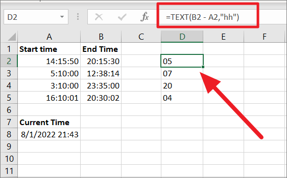
To get only the hours elapsed between the two times:
=TEXT(B2-A2,"hh")In the above, hh represents the hour unit. As you can see, the formula subtracts the time in B2 from A2 and then outputs only the numbers of hours elapsed between the start and end times.
Time Difference in Minutes between two times
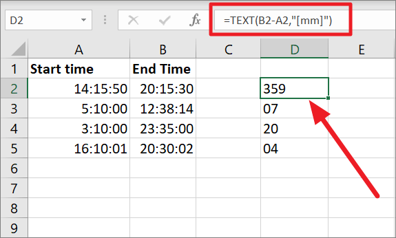
To get only the minutes elapsed between the two times, try this formula:
=TEXT(B2-A2,"[mm]")Where[mm] represents the total minutes. As you can see, the formula subtracts the time in B2 from A2 and then outputs only the number of minutes elapsed between two times.
Time Difference in Seconds between two times
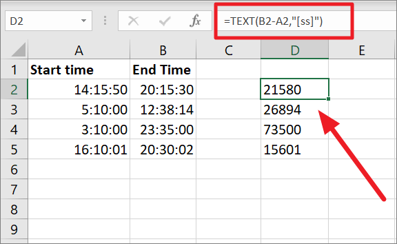
To get only the seconds elapsed between the two times, use this formula:
=TEXT(B2-A2,"[ss]")Where [ss] represents the total number of seconds. The formula subtracts the end time from the start time and returns only the total number of seconds.
You probably noticed the ‘mm’ and ‘ss’ formats are enclosed in square brackets, it’s because we want to get the total number of minutes or seconds between the two times and not just the remaining minutes or seconds besides hours. However, if the number of hours is more than 24 hours, you can use the ‘[hh]’ (enclosed in square brackets) format in the formula.
To find the remaining minutes between two times besides hours, use the below formula instead
=TEXT(B2-A2,"mm")To find the remaining seconds between two times besides hours, use the below formula instead
=TEXT(B2-A2,"ss")To return all three hours, minutes, and seconds between two times, use this formula:
=TEXT(B2-A2,"hh:mm:ss")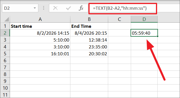
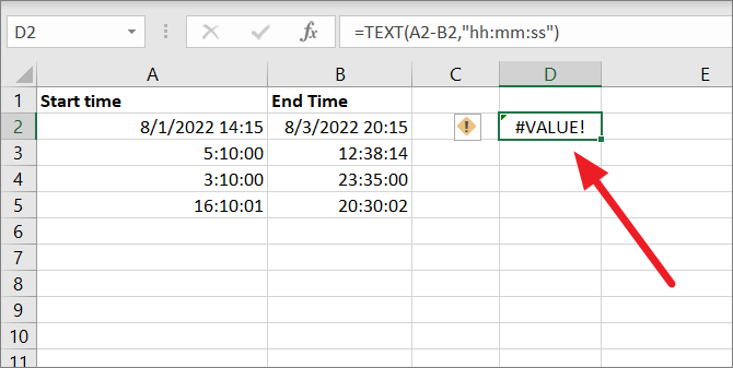
Note: The result returned by the TEXT function is always a TEXT. Hence, the output cannot be used in other calculations. If you intend to use the calculated time in other calculations, use any of the other methods to calculate the time difference.
If the returned value of the TEXT function is a negative number, you would get #VALUE! error.
Calculate Time Difference Between Two Dates
Before we start, you should know that Excel stores Data and Time as serial numbers. When you enter a Date in an Excel cell, it assigns a serial number, and if you enter a time, it assigns a fraction of a number.
Excel has a serial number system with dates starting from 1 Jan 1900 to this day and beyond. This means 1 Jan 1900 is 1, 2 Jan 1900 is 2, 3 Jan 1900 is 3, and so on. For example, the serial date number for the date 8/1/2022 is 44774 and the fraction or the decimal number for 6 AM is 0.25 (quarter day).
However, some earlier versions of Excel for Mac uses the 1904 date system. You also have the option to enable the 1904 date system. In such cases, the serial number will start at 1 Jan 1904 (0). And 2 Jan 1904 is 2, 3 Jan 1904, and so on.
Calculate Time Difference Between Two Dates in Hours
To calculate the time difference between two dates and times, you can use the below formula:
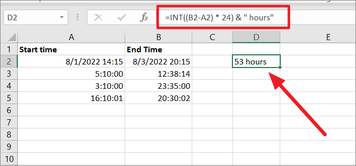
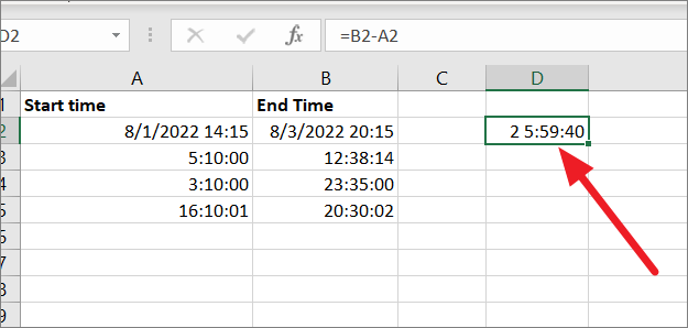
=INT((B2 – A2) * 24) & " hours"Where B2 is the End date and A2 is the start date. The Formula (B2-A2) will produce a fraction. We need to add the number of days + the fraction to get the difference in hours.
Let us see how this formula works:
As you can see the total difference between the two dates (when you applied ‘d h:mm:ss’ time formatting to the output cell) is 2 days, 5 hours, 59 minutes, and 40 seconds.
You can apply this custom formatting ‘d h:mm:ss’ in the Format cells dialog box.
Excel will calculate in terms of days and shows us there are 2 days of difference between the dates i.e 48 hours. This leaves us with 5 hours, 59 minutes, and 40 seconds. Now, we also need to add this into the output.
To do that, we need to convert the 5 hours, 59 minutes, and 40 seconds in terms of days. Since our time ends with seconds, we will calculate the 5 hours, 59 minutes, and 40 seconds in terms of seconds as shown below:
- 5 hours * 60 minutes * 60 seconds = 18,000 seconds
- 59 minutes * 60 seconds = 3,540
- 40 seconds
- 5 hours, 59 minutes, and 40 seconds = 18,000 seconds + 3,540 seconds + 40 seconds = 21,580 seconds.
To calculate the decimal for the day, we need to divide the above total of 21,580 seconds by 86,400 seconds (i.e. the total number of seconds in 1 day).
- 21,580 / 86,400 = 0.249769 days
As a result, the fraction we will get is 0.249769 days.
Now, the final difference between the two dates is 2 days + 0.249769 = 2.2497685.
Alternatively,
- The serial number for the Start DateTime (8/1/2022 2:15:50 PM) is 44774.59433.
- The serial number for the End DateTime (8/3/2022 8:15:30 PM) is 44776.8441.
- End DateTime (B2) – Start DateTime (A2) = 44774.59433 – 44776.8441 = 2.2497685.
To convert the above output into hours, multiply it by 24:
- 2.2497685 * 24 = 53.994444 hours.
Finally, the INT function trims the decimals at the end and the ‘&’ operator adds the text string (hours) at the end to give the total number of hours between the two days, which is ’53 hours’.
Calculate Time Difference Between Two Dates in Minutes
Calculating the time difference between two dates in Minutes is similar to calculating hours, the only difference is that you need to multiply the time difference by 1440 (number of minutes per day) in the formula. Then, add the ‘minutes’ text string at the end instead of ‘hours’.
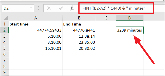
To calculate the time difference between two dates in terms of minutes:
=INT((B2 - A2) * 1440) &" minutes"Where B2 is EndDate and A2 is the StartDate. In the above formula, the subtraction output time difference between two dates is multiplied by 1440 (the number of minutes in 1 day). And then the string ‘minutes’ is appended to the result.
Calculate Time Difference Between Two Dates in Seconds
Calculating Seconds is the same as calculating hours and minutes, the only difference is that you will multiply the subtraction output by 86400 (number of seconds in a day).
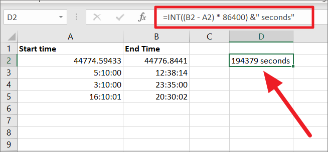
To do this, you can use the below formula:
=INT((B2 - A2) * 86400) &" seconds"The formula subtracts the Datetime in B2 from A2 and then multiplies the result by 86400 (number of seconds in a single day) because we want the result in terms of seconds. This will produce 194379 as the result. Since there are no decimal values, the INT function will return the same output (total number of seconds between two dates).
Calculate all Days, Hours, Minutes, and Seconds Between Two Dates
In case you want to get the time difference between two dates in terms of days, hours, minutes, and seconds, you need to use the TEXT function with the INT function.
To calculate Days, Hours, Minutes, and Seconds Between Two Dates, try the below formula:
=INT(B2-A2) & " days, "& TEXT(B2-A2,"h"" hours, ""m"" minutes, and ""s"" seconds""") 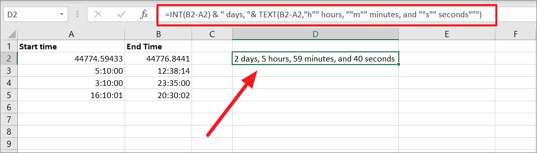
Here, the first part of the formula works the same way as in the previous examples. The INT function returns an integer value generated by subtracting the given dates (2.2497685) which is 2 days.
In the second portion of the formula, the TEXT function subtracts both dates and then applies custom number formatting to the result (5:59:40 AM). The "h" format returns the number of hours, "m" returns the number of minutes, and "s" returns the number of seconds. The TEXT function also adds the strings in double quotes hours, minutes, and seconds after every time unit.
Finally, both the INT and TEXT functions outputs are combined together using the concatenation operator (&) operator to give this result: 2 days, 5 hours, 59 minutes, and 40 seconds.
As you may have noticed, we added a space after every text string in the formula. Make sure to add those spaces to prevent results from getting jumbled up together.
Alternatively, you can also use the INT function with separate HOUR, MINUTE, and SECOND functions to get the same results:
=INT(B2-A2) & " days, " & HOUR(B2-A2) & " hours, " & MINUTE(B2-A2) & " minutes and " & SECOND(B2-A2) & " seconds"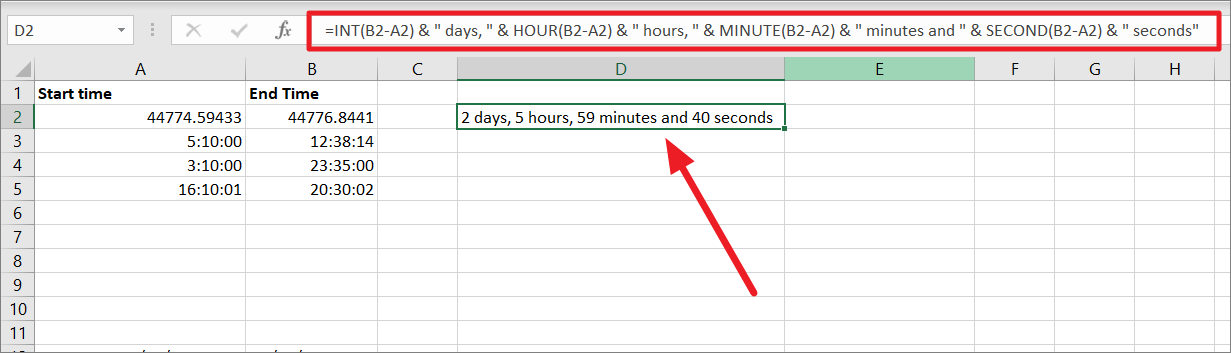
Subtracting Hours, Minutes, or Seconds from a Specific Time
Sometimes, we may want to subtract certain time intervals (Hours, Minutes, Seconds) from a specific time or DateTime. You can achieve this with or without the TIME function in Excel. If the hours you want to subtract are less than or equal to 23, you can use the TIME formula. But there’s another formula that can be used to subtract any number of hours.
Subtracting Any Hours from a Time without TIME function
For instance, if you have a particular date time and you want to calculate a time that was a certain number of hours before, you can divide the hours you want to subtract by the total number of hours (per day) and then subtract the result from the given time.
=Given Time/DateTime - (Hours to be subtracted/24)Example:
=A2 - (18 / 24)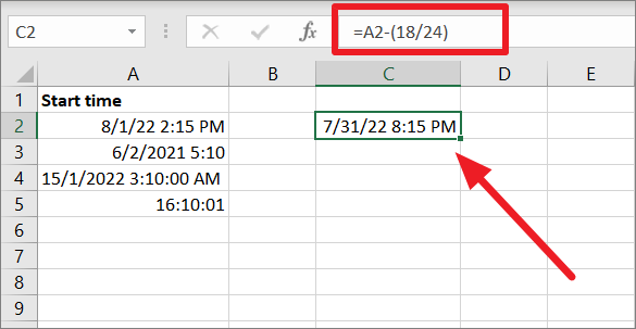
Here’s how the formula works:
Excel calculates the difference in terms of days, so we need to provide Excel with the number of days (or fraction) days we want to subtract from the given date or time (A2).
To calculate days, you must divide the hours your want to subtract by 24 (total number of hours per day) – 18/24. This will give us 0.75. If you want to subtract more than 24 hours, the number before the decimal point represents days and the value after the decimal represents time.
Now Excel will subtract 0.75 from the (44774.59433) which is the serial number for 8/1/2022 2:15:50 PM (A2) because Excel thinks in terms of fractions and decimals.
This will return 44773.84433 which is the serial number for ‘7/31/22 8:15 PM’. Hence, the output is 7/31/22 8:15 PM.
Example 2:
Let’s assume you want to go back 42 hours in time from August 1, 2022, 6:00 PM. So we need to provide Excel with the number of days we want to subtract from the given time.
To convert the hours into days, we need to divide 42 by 24 and then subtract it from A2:
=A2-(42/24)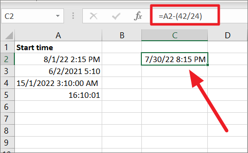
By dividing 42 by 24, we will get 1.75 days. As we mentioned earlier, the number before the decimal represents days (1) and the fraction after the decimal represents hours (0.75).
When multiplying 0.75 by 24 (0.75*24), we will get 18 hours. So, Excel will subtract 1 day 18 hours from A2 (August 1, 2022, 6:00 PM). The final output is 7/30/22 8:15 PM.
While the above simple arithmetic formula can be used for any number of hours from the given time, you can use the TIME formula if the hours to be subtracted are less than or equal to 23.
Subtracting Hours from a Time using the TIME function
TIME function allows you to convert a single time value into the individual hour, minute, and second units. It can also be used to merge individual time units into a single time value. However, the TIME function can only handle up to a maximum of 23 hours, 59 minutes, and 59 seconds.
Syntax:
= Given Time/DateTime - TIME(Hours to be subtracted, 0, 0)Example:
To go back 18 hours in time from August 15, 2022 evening (6 PM), use the following TIME formula:
=A2 – TIME (18, 0, 0)The TIME function has three arguments – hour, minute, and second. We want to subtract 18 hours, so the first argument is ’18’, and the other two arguments – minute and second are specified as ‘0’.
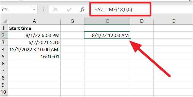
Usually, TIME function returns an output between 0 (0:00:00 or 12:00:00 AM) to 0.99988426 (11:59:59 P.M.). In the above formula, it returns 0.75 which is subtracted from A2.
Subtracting Minutes from a DateTime
We can use the same above formulas for subtracting minutes and the only difference is that we need to divide the minutes to be subtracted by 1440.
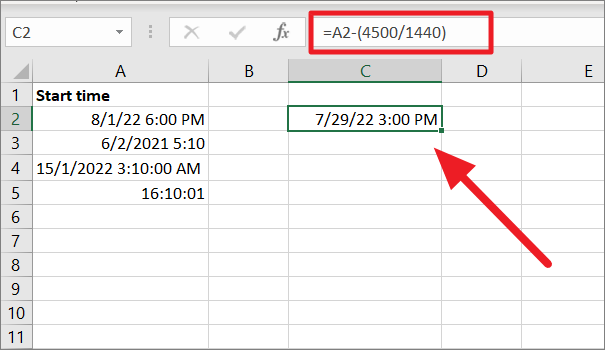
= A2 - (4500/1440)In the above formula, the number of minutes we want to subtract (4500) is divided by the total number of minutes in 1 day (1440) to convert minutes into days. The division will return 3.125 days which when subtracted from A2, and we will get the output of ‘7/29/22 3:00 PM’.
Subtracting Minutes from a Specific Time using the TIME function
You can also use the TIME function to subtract minutes from a specific time as long as the time to be subtracted is less than or equal to 1439 because of the TIME function limitation. It can only handle up to 23 hours, 59 minutes, and 59 seconds which is a total of 1439 minutes. If you want to subtract more than 1439 minutes, you need to use the above arithmetic formula.
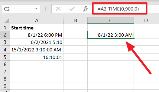
To subtract 900 minutes from the given time using the TIME function:
=A2 - TIME(0,900,0)In the above formula, the minutes (900) we want to subtract is is specified in the second argument of the TIME function. This gives us August 01, 2022, 3:00 am.
Subtract Seconds from a DateTime
We can use the same above formulas for subtracting seconds and the only difference is that the denominator in the bracket is 86400.
Syntax:
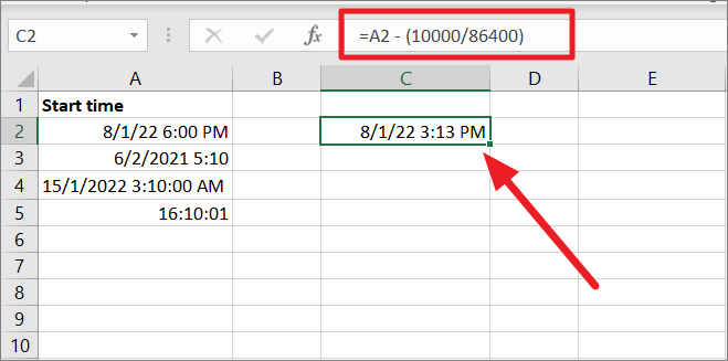
= A2 - (seconds to be subtracted / 86400)In the above formula, the number of seconds we want to subtract (10000) is divided by the total number of seconds in 1 day (24 hours * 60 minutes * 60 seconds = 86400) to convert seconds into days. The division will return 0.115740741 days which when subtracted from A2, we will get ‘8/1/22 3:13 PM’.
Subtracting Seconds from a Specific Time using the TIME function
Once again, you can also use the TIME function to subtract seconds from a specific time as long as the time to be subtracted is less than or equal to 86399 because of the TIME function limitation. It can only handle up to 23 hours, 59 minutes, and 59 seconds which is a total of 86399 minutes. If you want to subtract more than 86399 seconds, you need to use the above arithmetic formula.
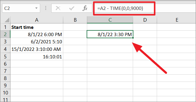
To subtract 9000 seconds from the given time using the TIME function:
=A2 - TIME(0,9000,0)In the above formula, the seconds (9000) we want to subtract is is specified in the second argument of the TIME function. This gives us August 01, 2022, 3:30 pm.
Subtracting Hours, Minutes, and Seconds from a Specific Time using the TIME function
If you want to subtract hours, minutes, and seconds from a certain date time, the TIME function can help.
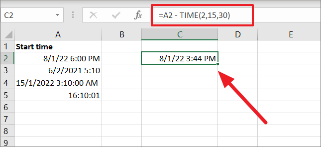
For example, to subtract 2 hours, 15 minutes, and 30 seconds, try the below formula:
=A2 - TIME(2,15,30)In the above formula, we specified all three-time units – hours, minutes, and seconds in the TIME function arguments. So, the formula subtracts 2 hours, 15 minutes, and 30 seconds from A2 (8/1/22 6:00:00 PM). This will give us 8/1/22 3:44 PM.
Calculating Negative Times in Excel
When subtracting time if the End Time is lower than the Start Time, then you will get a negative number in the time difference. The formula will result in negative numbers if the time difference is less than 0. This usually happens, when you input only times into a spreadsheet without dates.
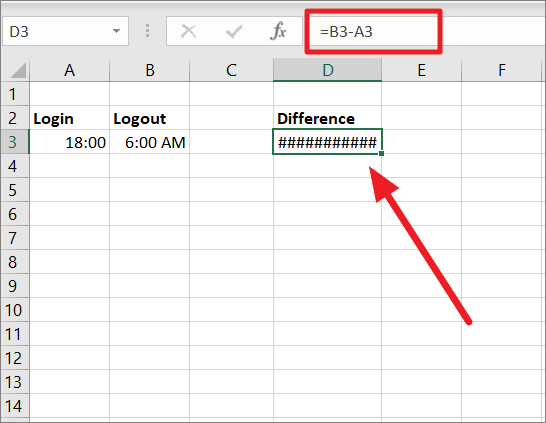
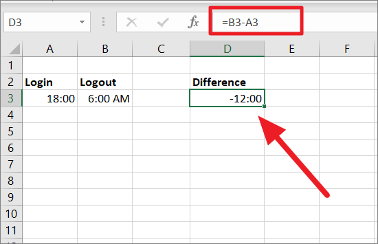
Also, if you usually work at nightshift, the end time and date will always be earlier than the start date and time of your work. For example, if you start your work at 6 PM and then finish your work and log out the next morning at 6 AM, the regular subtraction method won’t work.
As you can see below, not only the formula won’t, Excel will throw you the ###### error when you have a negative time.
However, if you want to display the negative anyway, you can just switch to the 1904 date system. Most modern Excel version defaults to the 1900 date system but if you change the date system to 1900, you can display the negative time values.
Here’s how you can switch to the 1904 date system in MS Excel:
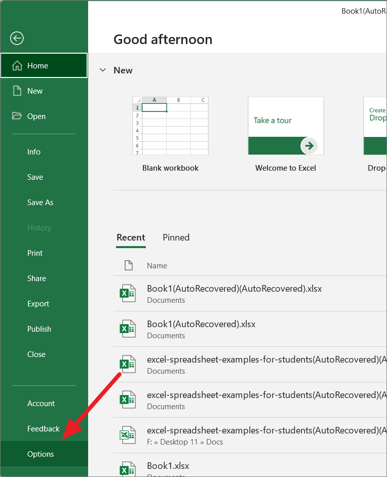
To do this, Click the ‘File’ menu on the Excel window and then select ‘Options’ in the backstage view.
In the Excel Options window, go to the ‘Advanced’ tab on the left, and then scroll down to the ‘When calculating this workbook section’. Then, check the box for ‘Use 1904 date system’ and click ‘OK’.
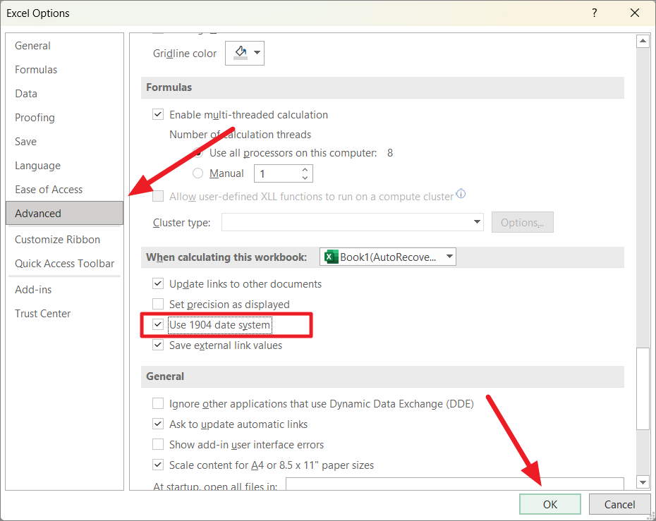
Now, Excel will display the negative date and time values as shown below:
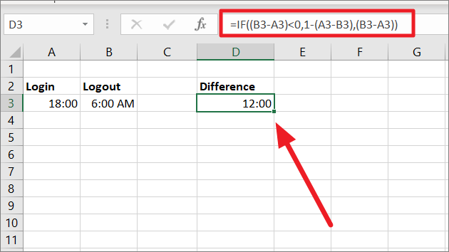
If you want to display time in negative values, you can use the IF function to force negative times to display properly.
You can use either of the following formulas to display negative times properly when times cross midnight:
=IF((B3-A3)<0,1-(A3-B3),(B3-A3))or
=IF(B3>A3,B3-A3,1-A3+B3)The above formula will calculate the negative time difference and display it properly as shown below.
However, the above formula will work in most cases. If the time difference is more than 24 hours, the above formulas won’t work either. In such cases, make sure to include dates with the times.
Subtracting the Dates to Count Days in Between
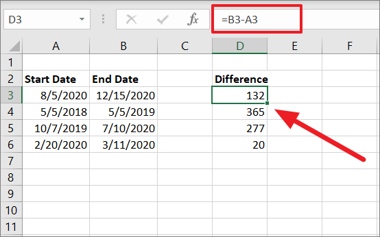
Similar to time, you can also subtract two cells with dates to find the number of days in between two dates.
For example, cell A3 and B3 contains two dates. To find the difference in days, use the below formula:
=B3-A3The formula returns the difference between two dates A3 and B3 as 132 days.
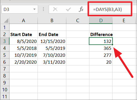
Count Days in Between Two Dates using the DAYS function
Besides the simple subtraction of cells, you can also use the DAYS function to calculate the difference between two dates.
The syntax
=DAYS(End date, Start Date)Example:
=DAYS(B3,A3)Where B3 is the End Date and A3 is the Start Date.
That’s the end. Now you know everything you need to know about substracting time in Excel and then some. Hopefully, knowledge of these functions will increase your productivity in Excel.


