How to Calculate Compound Interest in Excel

Albert Einstein once said, “Compound interest is the eighth wonder of the world. He who understands it, earns it; he who doesn’t, pays it.”

Compound Interest may be one of the most powerful financial concepts in the world but it’s not that hard to calculate and Excel makes it even easier. Compound Interest is a concept in finance that refers to the interest on a loan or deposit calculated based on both the initial principal and the accumulated interest from previous periods.

Think of it this way: if you put some money in a savings account that pays compound interest, each time you earn interest, that interest is added to your account balance. So the next time interest is calculated, it will be based on a higher balance, and you will earn more interest. Over time, this leads to much faster growth compared to simple interest. Compound interest is used in various financial products such as savings accounts, certificates of deposit, bonds, and other investment vehicles.

In this tutorial, we’ll explain how to calculate simple compound interest, reverse compound interest, and continuous compound interest with examples in Excel. We will also show you how to create a compound interest template or calculator for different compounding frequencies.

Simple Interest vs Compound Interest

Simple Interest and Compound Interest are two different methods of calculating interest on a loan or investment. The main difference between the two is how the interest is calculated and added to the principal amount over time.

Simple Interest: Simple interest is calculated based only on the principal amount and the interest rate. Simple interest does not compound, so the interest earned in each period is not added to the principal, and therefore, the balance does not grow as quickly as with compound interest.

Compound Interest: Compound interest is calculated based on both the principal and the accumulated interest from previous periods. With compound interest, the interest earned in each period is added to the principal, so the balance grows faster over time.

In conclusion, compound interest results in faster growth of wealth or debt compared to simple interest, due to the reinvestment of interest earned.

Calculating Compound Using Operators in Excel

Let us see how to calculate compound interest in Excel with a simple arithmetic formula to get a better idea of how compounding works. In the subsequent section, we will get down to calculating the future value of the investment on different compounding periods but first, we will see how your investment increases every year, month, quarter, etc. when calculating compound interest.

Annual Compound Interest with Arithmetic Formula

Suppose, you are investing $100 at an annual interest rate of 5% and now you want to know how your investment grows year-on-year with compound interest, here’s the formula you can use:

=Principal Amount * (1 + Interest)

In our example, the formula is:

==B1*(1+$D$1)

Where B1 is the initial investment i.e. $100 and $D$1 is the interest i.e. 5%. As you can see, we fixed the reference to cell D1 with the $ sign because the interest remains the same every year and so it doesn’t change as we copy the formula in the next step.

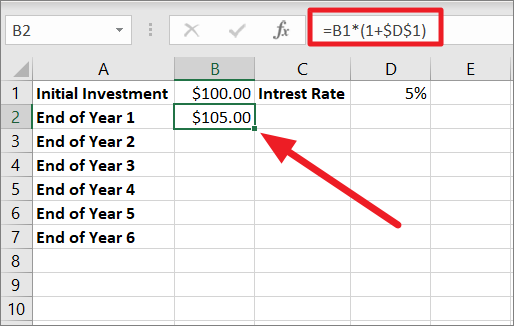
Excel stores percentages as decimal values, so percentages from 0% to 100% are equivalent to decimal values from 0 to 1. For instance, 1% is one part of 100 i.e. 0.01, so this means 5% is 0.05. Here, the interest is compounded once per year, hence (1+$D$1) or (1+0.05). So, after 1 year, your investment grows to $105.

Now, we need to calculate the balance after 2 years. To do that, we will use the ‘End of Year 1’ balance i.e $105 to calculate the compound interest at the same interest rate. This can be done by copying the same formula down to cells B3, B4, B5, etc. Drag the Fill handle to copy the formula.

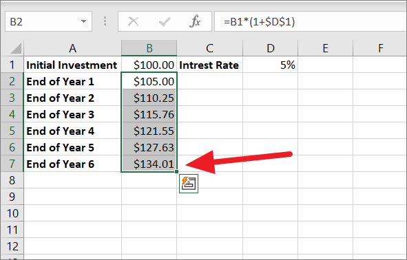
At the end of year 6, the invited amount is increased to $134.01.

This can also be calculated by multiplying the initial amount of $100 by 1.05 for every year. Then, round up the value to two decimal places, and you’ll get the same result.

To get the balance after 6 years, multiply $100 by 1.05 six times:

=100*1.05*1.05*1.05*1.05*1.05*1.05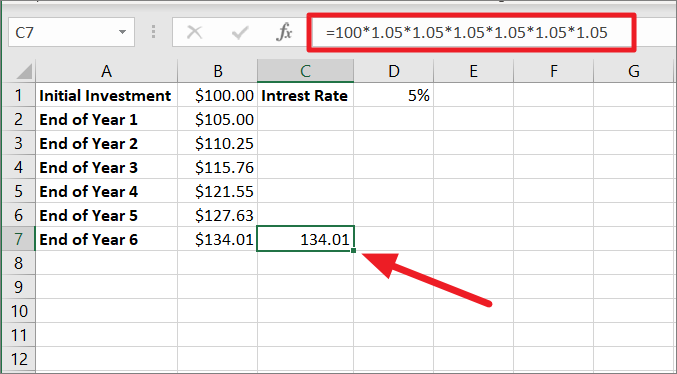

Compound Interest Rate Formula

The syntax for calculating the compound interest is,

Compound Interest = Final Amount - Initial Amount

If you wish to calculate the total interest you earned with compounding, simply subtract the initial amount (B1) or the start amount from the final amount or future value(B7).

=B7-B1 
=134.01-100 =34.01

The compound interest accumulated over six years is 34.01.

The above formulas show how simple compounding interest works in Excel. However, when it comes to calculating the future value of your investment, these formulas are inadequate. Besides, you cannot use these formulas to calculate the future value (final value with different compounding periods – daily, weekly, monthly, quarterly, or half-yearly.

Mathematical Compound Interest Formula for Different Compounding Periods

There is another simple mathematical formula you can use to calculate how much money you will earn when compounding yearly, quarterly, monthly, weekly, or daily. Fortunately, this formula doesn’t require you to create an entire table, you can just calculate the future value by specifying the duration and interest rate.

To calculate the final amount or future value with the compound interest we will need the initial principal amount, interest rate, compounding frequency, and the number of years.

Syntax:

The syntax is as follows:

FV = PV * (1 + R/N)^T*N

Where

FV – The future or final value of the investment after compound interest is applied.
PV – Present Value refers to the initial amount or principal amount invested. When specifying a percentage, you can use percentage, decimal, or fraction. For example, 10% can be specified as 0.1 or 10/100.
R – Annual rate of interest.
N – The number of times compounding occurs per year (e.g. 1 for yearly, 4 for quarterly, 12 for monthly, etc.).
T – The number of years over which compound interest is applied.

Now, we can use the above compound interest formula for calculating the final value or future value of your investment with different compounding frequencies:

yearly compounding,
quarterly compounding,
monthly and weekly compounding,
daily compounding.

Yearly Compounding with Mathematical Formula

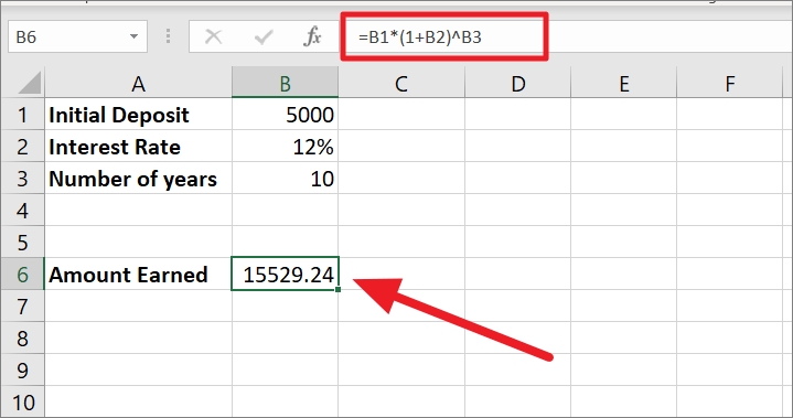
Let’s assume you are making a deposit of 5000 into a savings account and the bank offers an interest rate of 10% that is compounded yearly. Now, you want to know how much you will get in return after 10 years. This is the formula you will use for yearly compounding:

=B1*(1+B2)^B3

=B1*(1+B2/1)^B3*1
=5000 * (1+12%/1)^10*1
=5000 * (112%)^10
=5000 * 3.105848
=15529.24

Since it is a yearly compounding, the interest is compounded only once per year. Hence, the interest rate of 10% is divided by 1. Then, it is added to 1 which returns 1+12% equals 112% (1 is 100%, so 1+12% = 112%).

After that, the caret symbol (^) is used to raise the number or give exponents. The 112% is raised to the power 10 (10*1) as the number of years which results in 3.105848%. Finally, 5000 is multiplied by 3.105848 to get the future value of 15529.24. This is the final amount earned on the initial deposit of 5000 after 10 years at a 12% interest rate.

This formula is similar to the one used by banking and financial institutions for calculating compound interest.

To find the interest earned by the initial deposit, subtract the initial amount from the final amount:

Compound Interest = Future Value - Initial Value

Compound Interest = 15529.24 – 5000

Compound Interest = 10529.24

Half-yearly Compounding with Mathematical Formula

Now, let us see how to calculate half-yearly compounding. For half-yearly compounding, the interest is compounded every six months which makes the number of times the interest is compounded 2 times per year.

To calculate compound interest half-yearly, you only have to change the N value (Number of times interest is compounded) in the same formula:

=B1*(1+B2/2)^(B3*2)

You can use also write the formula like this by referencing the cell containing the value for the N argument instead of directly specifying the value:

=B1*(1+B2/2)^(B3*2)

Since the interest is compounded twice a year here, the 12% interest rate is divided by 2 which gives us 0.06. Then 1 is added to 0.06 equals 1.06. The number of years (10) is multiplied by compounding times (2) and the result (20) is used as the exponent.

The 1.06 is raised to the power 20 which produces 3.207135472. Finally, 3.207135472 is multiplied by the principal balance of 5000 which results in 16035.68.

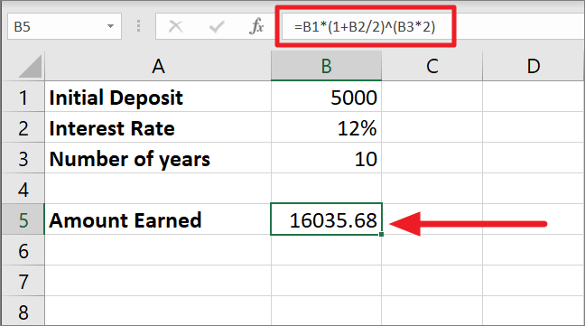
As you can see the amount earned for half-yearly compounding is slightly higher than the yearly compounding. The more frequent the compounding period, the higher the future value will be.

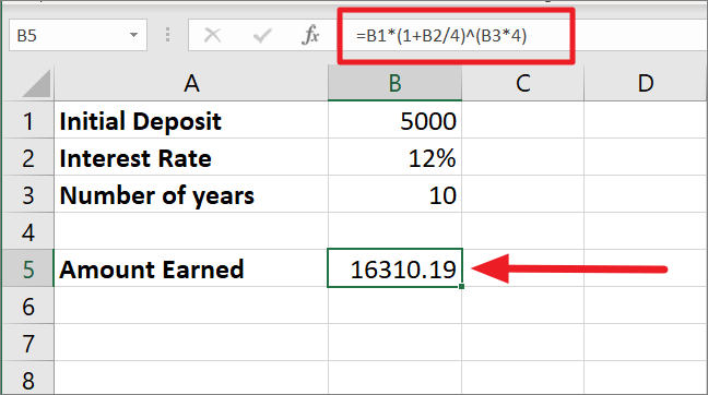
Quarterly Compounding with Mathematical Formula

In the case of monthly compounding, compound interest is applied every 3 months in a year, which makes the number of times the interest is compounded 4 times per year. Just like with the previous formula, the only thing we are changing here is the number of compounding times which is 4. Here’s the formula for calculating compound interest quarterly:

=B1*(1+B2/4)^(B3*4)

In this formula, the interest rate of 12% is divided by 4 and its result of 0.03 is then added to 1. This gives us 1.03 which is raised to the power 40 (10*4) because 10 is the number of years and 4 is the number of times interest is compounded in a year. With 1.03 as the base number and 40 as the exponent, we get 3.27. At last, multiplying 3.27 with the initial amount of 5000 gives us the final amount of 16310.19.

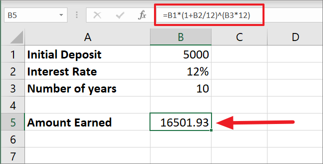
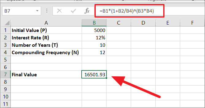
Monthly Compounding with Mathematical Formula

Now, move let us move on to the Monthly Compounding. For half-yearly compounding, the interest is compounded every month of the year so naturally, the number of times the interest is compounded is 12 times in a year.

In the below formula, we only need to change the N value (Number of times interest is compounded) to find month compounding:

=B1*(1+B2/12)^(B3*12)

Since the interest is compounded every month of the year, the 12% interest rate is divided by 12 which gives us 0.01. Then 1 is added to 0.01 equals 1.01.

Then 1.01 is raised to the power 120 (10*12) as 120 is the total number of times interest will be compounded in the duration of 10 years. With that, we are at 3.300387. Finally, 5000 is multiplied by 3.300387 which gives us the final balance of 16501.93.

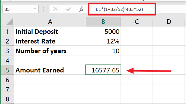
Weekly Compounding with Mathematical Formula

If you want to find weekly compounding for the initial amount, you can use the formula in this section. When it comes to calculating the compounding interest weekly for the investment value the number of times the interest is compounded in a year becomes 52.

Here’s the formula for weekly compounding, run the below formula in Excel:

=B1*(1+B2/52)^(B3*52)

Since the interest is compounded every month of the year, the 12% interest rate is divided by 52 which gives us 0.002308. Then 1 is added to 0.002308 equals 1.002308.

Then 1.002308 is raised to the power 520 (10*52) as 520 is the total number of times interest will be compounded in the duration of 10 years. By multiplying the rate and number of periods, we get 3.316059. Finally, 5000 is multiplied by 3.316059 which makes the final amount to be 16577.65.

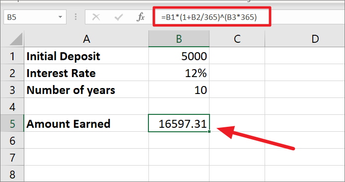
Daily Compounding with Mathematical Formula

Daily Compounding gives you a higher return on your investment or deposit than other compound interests. In the daily compound interest method, the daily interest is earned on your investment after interest from the previous day is added.

For daily compounding, the interest is compounded every day of the year which makes the number of times the interest is compounded 365 times in a year. Here’s the formula for daily compounding in Excel:

=B1*(1+B2/365)^(B3*365)

In daily compounding interest is compounded 365 days a year, so the interest rate is divided by 365. Then, the adjusted interest rate 1 is added to the divided value which returns 1.032877.

Now, 1.000328767 is calculated at the power 10*365 (number of years time number of compounding periods) which equals 3.31946071. Finally, 3.31946071 is multiplied by $5000 which makes the final amount $16597.31.

Compound Interest formula Template in Excel

Instead of creating different formulas for different compounding periods, you can create an all-in-one excel template that helps to calculate compound interest no matter what your compounding periods are. Here’s the compound interest calculated for different compounding periods:

=B1*(1+B2/B4)^(B3*B4)

The above formula is not that different from the previous formulas, but the only difference is that we referred to B4 as the N argument (number of times compounding occurs). Instead of manually entering the N argument in the formula, you can just change the compounding frequency in cell B4 (e.g. 4, 12, 52, etc.) and use the same formula for calculating compound interest with different periods.

Calculating Compound Interest using FV Function in Excel

As we mentioned before, there are no Compound Interest formulas in Excel. But you can use functions like FV() function to calculate compound interest and final value. The FV function, short for Future function is used to calculate the future value (initial investment + compound interest) of an investment based on constant payments and interest rates. As with mathematical formulas, you can also use FV() function to calculate yearly, quarterly, monthly, weekly, and daily compounding.

The Syntax

Here’s the general syntax for FV() function:

=FV(rate, nper, pmt, [pv], [type])

The arguments:

rate – The constant interest rate to be applied to an amount for each period.

nper – The total number of compounding periods that occurs per year. It can be monthly, quarterly, monthly, yearly, etc.

pmt – The additional payments made each period; must be a negative number. If no amount is paid, then put 0 as its value. If this value is omitted, then provide the PV argument.

pv (optional) – This represents the present value of the investment or loan. It must be represented as a negative number. If omitted, it defaults to 0 (zero).

type (optional) – This specifies whether payments (EMI) are made at the start of the period or the end of the period. If the EMI is paid at the start of the period, enter 0 or enter 1 if the EMI is paid at the end of the period. If omitted, it defaults to 0.

Now, we understand the FV function and its arguments, let us use it in a few examples.

Suppose, you are investing 2000 dollars for 5 years at an annual interest rate of 6%. Let’s calculate the future values of investment in different compounding periods.

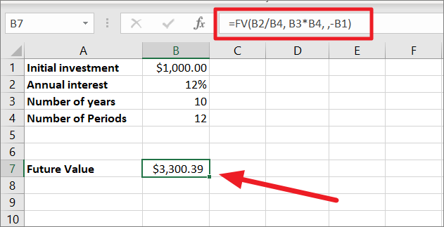
Monthly Compounding with FV function

First, let’s calculate the future value of an investment that is compounded Monthly with no additional payments. Here’s the compound interest formula:

=FV(B2/B4, B3*B4, ,-B1)

In the above formula:

The value of the rate parameter is B2/B4 i.e. 12/12 or 0.012/12 because the 12% interest rate is compounded monthly (12).
For nper, we are multiplying 5 years by the number of compounding periods. i.e. 10*12.
We left the pmt blank because we are not making any additional payments.
Since we left the pmt argument empty, we are required to specify the pv argument. Since B1 is our initial value, we refer to it as the PV argument. It is represented as a negative number because its an outflow.

Now, let us see how the FV compound interest formula works with additional payments. You can extend the above formula’s capacity by adding pmt argument.

=FV(B2/B4, B3*B4,-B5,-B1,B6)

The only difference between this formula and the previous formula is the addition of the ‘additional payments’ argument. Since we are making additional contributions of 200 to the present value, enter the additional payment or refer to the cell with the value in the formula. When we add the additional payment to the formula, you should also specify the additional argument type. Enter ‘1’ if you make additional payments at the beginning of the compounding period or type ‘0’ if the payments are made at the end of the period.

First, add the necessary values to the table and adjust the formula accordingly as shown below. As you can see, additional payments will significantly increase the future value.

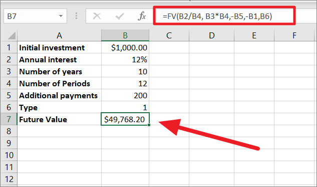
To get only the interest earned through compounding, you just need to subtract the initial investment from the final value:

=Future value - initial value

=49,768 - 1000
=48,768

The compound interest earned from the initial amount for 10 years, and the monthly compounding period is 48,768.

Now, we use can the same FV formulas for all the compounding periods – daily, weekly, monthly, quarterly, or yearly. We don’t need to change anything in the formula, the only thing you need to change is the value of the ‘Number of Periods’ (Compounding Frequencies) in the table and the result will automatically adjust.

Advanced Compound Interest Template/Calculator for all Compounding Frequencies

Instead of writing different formulas every time you want to compute compound interest, you can create an advanced Computer Interest calculator that can be used for all purposes no matter what your compounding periods are. Here’s how you do that.

First, create a table with necessary data (initial amount, annual interest rate, total years of investment) as shown below. Type the labels – Initial investment, Annual interest, number of years, and Compounding periods in column A. Then, enter the corresponding values in column B. But leave the cell (B5) adjacent to compounding periods empty, we are going to create a drop-down list for that.

In case you are making additional payments to the investment, you will need to add an additional payment label and its value to the above table.

Now, let’s create a drop-down for the number of compounding periods per year, so you don’t have to manually input numbers every time.

To do that, create another table next to the first table with the name of the compounding frequencies as headers and the number of periods as values (as shown below).

Next, we need to create a table with the periods range. To do that, select the newly created data range (D2:I3), go to the ‘Insert’ tab, and select ‘Table’ or just press Ctrl+T.

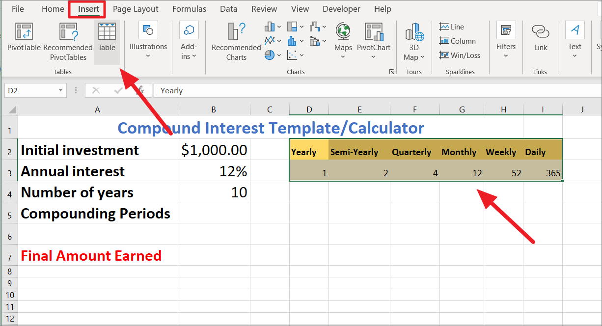
In the Create Table dialog box, confirm the range, make sure the ‘My table has headers’ option is checked, and click ‘OK’.

Then, anywhere on the table, switch to the ‘Table Design’ tab, and give a name to the table in the ‘Properties’ section of the Ribbon. In the below example, we are naming the table ‘Table2’. You can also choose to remove the filter button by unchecking the ‘Filter Button’ in the ‘Table Style Options’ group.

After that, select the cell adjacent to the ‘Compounding periods’, go to the ‘Data’ tab in the ribbon, and select the ‘Data Validation’ button in the Data Tools group.

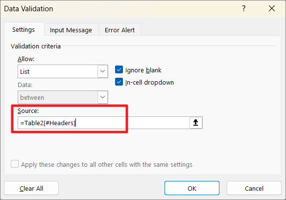
When the Data Validation dialog opens, select ‘List’ under the Allow drop-down menu.

In the ‘Source:’ field, refer to the header of the compounding frequency table with this syntax:

=Table_Name[#Headers]

[#Headers] is used to refer to the header row (column headers) of the table. E.g. =Table2[#Headers].

Or, you can just click on the Source field and just select the range (column headers) from the worksheet. Then, click ‘OK’.

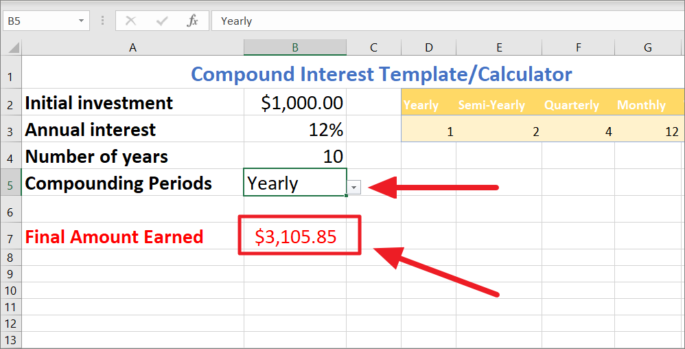
Now, you have a drop-down list with compounding frequency names.

Next, type your Compound interest formula where you want the result (B7).

=FV((B3/HLOOKUP(B5,Table2[#All],2,0)),(B4*HLOOKUP(B5,Table2[#All],2,0)),,-B2)

In the above formula, we are using the HLOOKUP formula to divide the annual rate (B3) and multiply the number of years (B4). The HLOOKUP function searches ‘Table2’ for the exact value in ‘B5’ and retrieves a corresponding value in the same column from the 2nd row.

Here, the Compounding period is selected as Monthly, so the FV function uses HLOOKUP to look for the ‘Monthly’ value in the ‘Table2’ header and return the corresponding value from the 2nd row in the same column. i.e. 12 periods. Then, the FV function uses the retrieved compounding period (12) to calculate the future value (Initial investment + compound interest) which is $3,309.39.

Now, simply change the compounding periods to get different future values. You can use the template to calculate compound interest for any value. All you have to do is change the input values in cells B2, B3, B4, and B5.

The above template can be downloaded here.Download

Calculate Intra-year Compound Interest Using the EFFECT Function

The EFFECT function in Excel calculates the effective annual interest rate from the nominal interest rate. EFFECT can be useful for comparing financial loans with different compounding terms. Intra-year compound interest means interest that is compounded more frequently than once a year.

The Syntax of EFFECT function:

=EFFECT(nominal_rate, npery)

Where:

nominal_rate: The nominal interest rate, expressed as a decimal.
npery: The number of compounding periods per year.

For example, to calculate the annual interest rate of a nominal rate of 5% compounded quarterly, you use this formula:

=EFFECT(8%, 4)

It would return 0.0506, which represents 5.06% as the effective annual interest rate. Now, the above EFFECT function can be used to build effective compound interest formula.

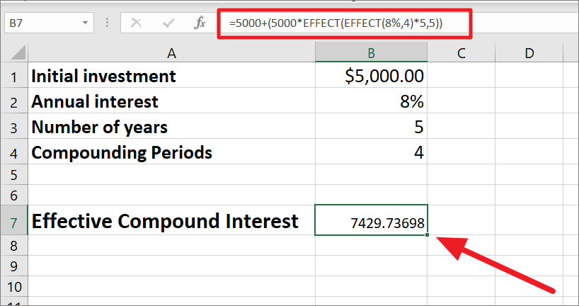
To calculate effective compound interest using the EFFECT function, use the following syntax:

=P+(P*EFFECT(EFFECT(R,N)*T,T))

Where

P – principal amount

R – Rate of interest

N – number of times compounding occurs per year (periods)

T – number of years

Example:

=5000+(5000*EFFECT(EFFECT(8%,4)*5,5))

Here, the principal is $5000, so we enter P=1000, and the interest rate is 8%, so R=8%. The compounding frequency is 4 for quarterly compound interest i.e. N=4. The Effect function is repeated 4 times, one of them is nested for annual compounding periods and then multiplied by 4 to spread out the compounded rate over the year.

Calculate Compound Interest with Different Interest Rate Using the FVSCHEDULE function

The FVSCHEDULE function in Microsoft Excel can also be used to calculate the future value of an investment based on a series of compounded interest rates. The formula for the FVSCHEDULE function is:

FVSCHEDULE(principal, schedule)

where:

principal: the initial amount of the investment
schedule: an array or range of interest rates that represent the interest rate for each period of the investment. The array can contain any number of interest rates.

Example: Let us assume you are making an investment of $1,000 that earns 5% interest in the first period, 6% interest in the second period, and 7% interest in the third period. Now, let us calculate the future value of that investment.

Here’s an example of using the FVSCHEDULE function to calculate the future value of an investment:

=FVSCHEDULE(B1, B2:B4)

Where B1 is the principal value and B2:B4 is the range of interest rate.

If you want to directly input the values into the formula, here’s an example:

=FVSCHEDULE(2000, {0.05,0.07,0.09})

The interest rates must be separated with commas and placed in curly braces.

Here’s how the formula works:

In the first period, the investment earns 5% interest, so the future value is $2,000 * (1 + 0.05) = $2,100.
In the second period, the investment earns 7% interest on the $1,050 balance, so the future value is $2,100 * (1 + 0.07) = $2,247.
In the third period, the investment earns 9% interest on the $1,110.30 balance, so the future value is $2,247 * (1 + 0.09) = $2,449.23.

However, if you were only given annual interest rates and compounding periods per year, then you need to compute the interest rate before using it in the formula.

To find the interest rate, divide the annual rate by compounding periods and store the values in a separate column.

Then, calculated interest rates are used to find the future value as shown below.

Calculate Reverse Compound Interest in Excel

As you know, you can easily compute compound interest with the principal investment, interest rate, and compounding periods. But, let’s say you only have principal value, compounding periods, and future value (initial value + total compound interest). Now, you want to find the compound interest rate. Here’s how you do this:

You can easily compute the compound interest rate with the final amount and initial principal, along with the number of compounding periods. The reverse compound interest rate formula is:

= (FA/PA)^(1/n) - 1,

Where

FA – final amount (including interest)
PA – principal amount
n – number of compounding periods

This formula calculates the interest rate given the final amount and initial principal, along with the number of compounding periods, by taking the nth root of the ratio of the final amount to the initial principal and then subtracting 1 from the result.

Example:

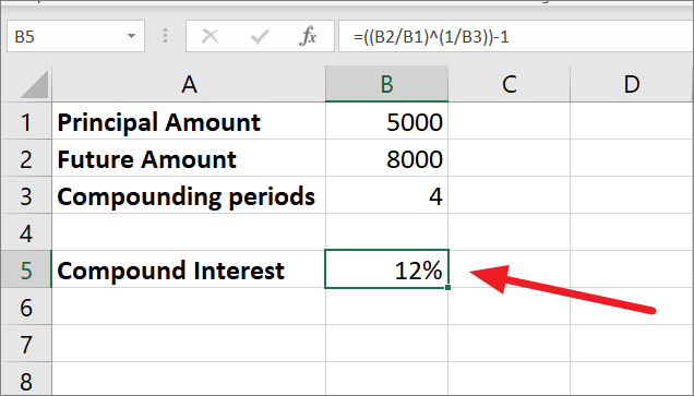
Suppose you have an initial investment of $5,000, and after 4 years the investment has grown to $8,000. To find the reverse compound interest rate:

=((B2/B1)^(1/B3))-1

The formula divides the final amount by the initial amount. Then it takes the 1/nth root of the result which results in 1.124683. Finally, 1 is subtracted from that to give us 0.124683. Now, the result represents the interest rate as a decimal.

To display it as a percentage, multiply it by 100 or select the result cell, click the ‘Number Format’ drop-down menu, and select ‘Percentage’.

So the reverse compound interest rate is 12%.

Calculate Reverse Compound Interest using the RATE function

The RATE function in Microsoft Excel can be used to calculate the reverse compound interest rate. The formula for the RATE function is:

=RATE(nper, pmt, pv, [fv], [type], [guess])

where:

nper: the total number of payment periods
pmt: the payment made each period
pv: the present value of the loan
[fv]: the future value of the loan (optional, default is 0)
[type]: the type of payment made (0 = end of period, 1 = start of period; optional, default is 0)
[guess]: an estimate of the interest rate (optional)

Here’s an example of using the RATE function to calculate the reverse compound interest rate:

=RATE(60, -200, 5000)

This example calculates the reverse compound interest rate for a loan. The loan has the following terms:

Total number of payment periods: 60
Payment made each period: -200 (negative sign indicates payments are being made)
Present value of the loan: 5000
Type of payment made: 0 (end of period)

The RATE function uses these inputs to calculate the interest rate required to achieve these payments and present value. This will return the interest rate as a decimal. Now, change the decimal to a percentage and you will get 3%.

Calculate Compound Interest with Regular and Irregular Deposits in Excel

So far we mostly focused on how to calculate the future value and compound interest on fixed one-time deposits or investments over certain periods. However, what if you want to calculate compound interest earned on a savings account or fixed deposit, where you make regular additions to the initial principal amount?

The interest earned on the initial amount, and each subsequent deposit, compounds over time resulting in a higher overall interest rate. This type of interest calculation can help increase the overall balance of the account and lead to greater savings over time. Let us see how to compute compound interest with regular and irregular deposits using the FV function and mathematical formulas.

Compound Interest with Regular Deposits using the FV function

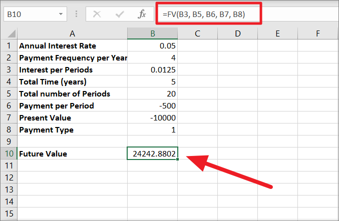
Suppose you have $10,000 as the present value (PV) of your investment and you want to invest for 5 years. The annual interest rate (r) is 5% and interest is compounded quarterly (n=4). You plan to make regular deposits of $500 every quarter.

The formula for the future value (FV) of an investment with regular deposits:

=FV(B3, B5, B6, B7, B8)

This formula uses the same syntax as the FV function we used before for calculating compound interest.

Where

rate – Interest per Period (B3) .i.e B1/B2 = 5%/4 = 0.0125
nper – Number of Periods (B5) .i.e. B2*B4 = 4*5 = 20
pmt – Payment per period (B6) = – 500
[PV] – Present Value (B7) = -10000
[type] – Payment type (B8) = 1. This specifies the payments are made at the beginning of the period.

The FV function calculates the future value based on the given input and displays it in cell B10 as 24242.89.

Calculate Compound Interest with Irregular Deposits Using Manual Formula

Unfortunately, you cannot use the same FV formula to calculate Compound Interest with Irregular Deposits. However, you can create a table to calculate compound interest with Irregular deposits. Here’s a step-by-step process for creating a table to calculate compound interest with irregular deposits:

First, create a table with columns for the periods (month number), the starting balance, the deposit made, and the ending balance as shown below. You can then add as many periods as you want under the Periods column. This is a quarterly compounding for 3 years, so a total of 12 periods.

Next, create another smaller table beside the first table with the Initial investment, annual interest rate, and compounding periods. Or you can also directly use these values in the formula. Then, calculate the interest rate by dividing the annual interest rate by the number of periods per year (cell G6).

Now, input your irregular deposit amount for each period under the ‘New Deposits’ column.

After that, in cell C2, enter this formula =G3+B2 under the Starting Balance column. This formula adds the investment to the calculation. Now, we got the balance at the start of the compounding period (New deposit + Initial investment).

Next, enter this formula, =C2+C2*(G6) in cell D2 (under the column Ending Balance). This formula adds Starting balance (C2) to the interest earned (C2*($G$6)) for the period.

Then, copy the formula and apply it to the cells below by dragging the fill handle. At first, you will get zeros in the column but they will be replaced later.

Next, enter this formula =D2+B3 in cell C3 under the column Starting Balance. This adds the New Balance to the Ending balance from the previous periods to create the Starting Balance for the next period. i.e. 11257.5.

Then, copy down the formula in cell D3 for other cells in the column. Now, the starting balance and ending balance have automatically updated in both columns.

The Future value for the investment with irregular additions is 19404.12.

Calculating Continuous Compound Interest in Excel

Compound interest calculates the interest of the principal and the accumulated interest over specific time intervals such as monthly, quarterly, semi-annually, and on annual basis. While Continous Compound interest is a method of calculating interest in which interest is compounded continuously over an infinite number of periods rather than a specific number of periods.

Continuous Compound Interest is used in a variety of financial applications and calculations including investment analysis, retirement planning, loan calculations, bond pricing, and financial modeling. Overall, continuous compounding is a useful tool for financial professionals to analyze and compare different investment options, make informed investment decisions, and plan for their financial future.

The formula for calculating the future value (FV) with continuous compounding is given:

FV = PV * e^(r * t)

where:

PV is the present value (initial investment)
t is the time period (in years)
r is the interest rate
e is the mathematical constant approximately equal to 2.71828

In this formula, the present value (PV) is multiplied by the value of ‘e’ raised to the power of ‘r * t’. Since the period is infinite, the variable ‘e’ is a mathematical constant used to describe the exponential growth, and the variable ‘r * t’ represents the interest rate multiplied by the time period. The result of this calculation is the future value of the investment, which takes into account the effect of continuous compounding over the specified time period.

Suppose you invest $10,000 for 5 years at an annual interest rate of 4% compounded continuously.

The future value can be calculated using the formula above:

FV = $10,000 * e^(0.04 * 5)

FV = $10,000 * e^0.2

FV = $10,000 * 1.221402758

FV = $12,214.03

So, after 5 years with continuous compounding, the future value of the investment will be $12,214.03. This means that your initial investment of $10,000 will grow to $12,214.03 after 5 years with interest being compounded continuously. Now, let us see the effects of continuous compounding on regular compounding.

Future Value for Annual Continuous Compound Interest

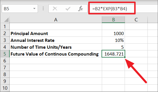
For example, if you invest $1000 at an annual interest rate of 5% for 5 years with continuous compounding, what will be the future amount after that period? Since Excel doesn’t recognize ‘e’ as a mathematical constant, we are going to use EXP() function to calculate the exponential value of the number.

=PV * Exp(r*t)

Where

PV = Present Value (the initial amount invested)
r = interest rate (as a decimal)
t = number of years the investment is held

Example:

=B2*EXP(B3*B4)

In the above formula, B2 is the Principal amount (PV), B3 is the rate of interest (r), and B4 is the number of time years (n).

The rate of interest is multiplied by the number of time units (10%*5=0.5), then the EXP function returns the value of the constant e raised to the power of the number (0.5). After that PV (1000) is multiplied by the value of the constant (1.648721) which results in the continuous compounding amount of 1648.721.

Future Value for Quarterly Continuous Compound Interest

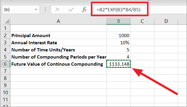
For example, if you invest $1000 at an annual interest rate of 5% for 5 years with continuous compounding, what will be the future amount after that period? Since its quarterly compounding, the number of years is divided by the number of compounding periods (4). Since Excel doesn’t count ‘e’ as a mathematical constant, we are going to use EXP() function to calculate the exponential value of the number.

=PV * Exp(r*t/n)

Where

n – Number of compounding periods per year.

Example:

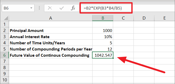
=B2*EXP(B3*B4/B5)

In the above formula, B2 is the Principal amount (PV), B3 is the rate of interest (r), B4 is the number of time years (n), and B5 is the number of compounding periods per year.

The number of time units is divided by the number of compounding periods (10%/4=1.25), then multiplied by the rate of interest. The EXP function returns the value of the constant e raised to the power of the number (0.125). After that PV (1000) is multiplied by the value of the constant (1.133148) which results in the continuous compounding amount of 1133.148.

Future Value for Monthly Continuous Compound Interest

If you want to calculate the future value (FV) with the monthly compounding interest for the same value and interest, use the below formula but change the compounding periods in the table:

=B2*EXP(B3*B4/B5)

In the above formula, B2 is the Principal amount (PV), B3 is the rate of interest (r), B4 is the number of time years (n), and B5 is the number of compounding periods per year.

Future Value for Daily Continuous Compound Interest

We are using the same formula for the Daily continuous compound interest but changing the number of compounding periods in the table. Unlike other compound interest calculations, as the number of compounding periods increases, the future value decreases when investment is compounded continuously.

=B2*EXP(B3*B4/B5)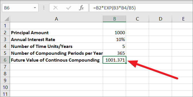

Calculate Compound Interest using What-IF analysis

You can also calculate compound interest using What-If analysis in Excel. What-If analysis in Excel is a tool used to analyze and evaluate the impact of different input values on a specific result. This can be done using a data table, which allows you to test multiple input values and see the corresponding outcomes in a grid format.

The data table can be a one or two-dimensional table, with the input values being changed in the row or column headers, respectively. The result of the formula can then be seen in the body of the table for each combination of input values.

One Variable Data Table to Calculate Compound Interest

A one-variable data table in Excel is a tool that allows you to see how changes in a single input value can affect a formula’s results. A one-variable data table can be used to calculate compound interest by changing the interest rate or initial amount and seeing how it affects the final amount. Here’s an example in Microsoft Excel:

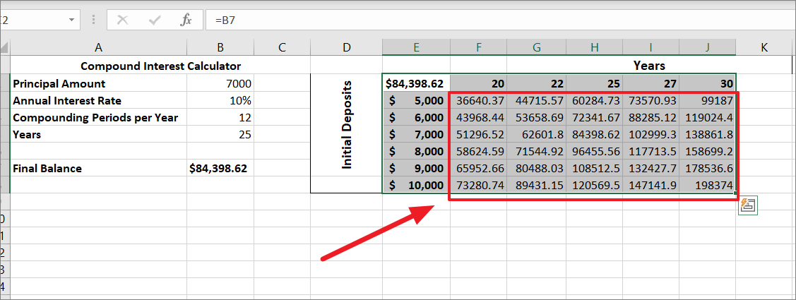
You just found out that there is a bank that offers an interest rate of 10% compounded monthly and you want to save $100,000 in 25 years. What should your initial deposit be in order to achieve this goal?

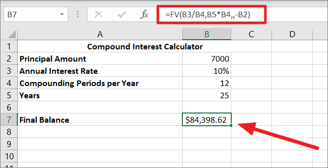
To test different values, first, we should build a compound interest calculator as shown below using the FV function:

=FV(B3/B4,B5*B4,,-B2)

In the below spreadsheet,

B7 contains the FV formula used to calculate the final or future balance.
B2 is the input value you want to test (initial deposit).

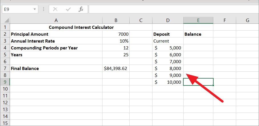
Now, let us do a What-If analysis using a one-variable data table to check what your savings will be in 25 years based on your initial deposit, ranging from $5000 to $10000.

To create a one-variable data table in Excel, follow these steps:

You need to create a data table for variable values and enter your values in one column or across one row. The table can either be column-oriented or row-oriented. In the below example, we entered our different input values in a column (D4:D9) and left one blank column beside it for the results.

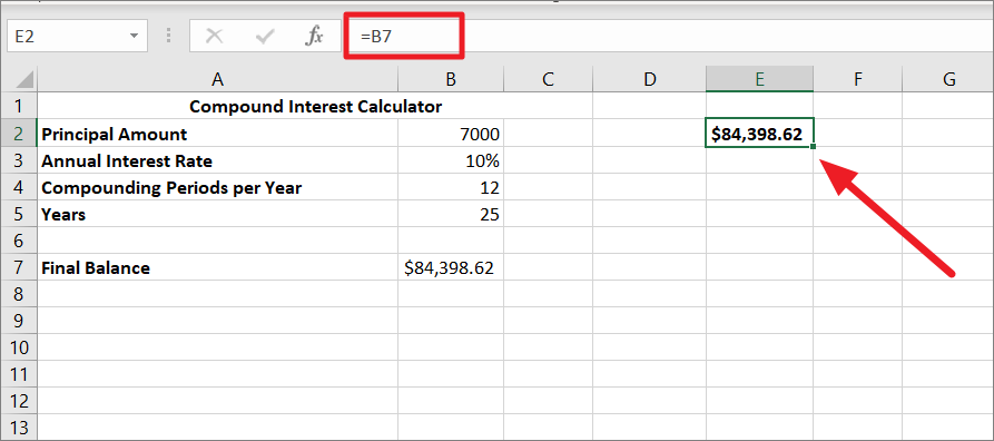
Next, type this simple formula =B7 in the cell one row above and one cell to the right of the variable values to link this cell to the formula cell in the original table. In our example, it’s cell E3. This way the results will be updated automatically in case you change the formula in the future.

However, you can also directly type your compound interest formula in E3.

After that, select the data table range containing your formula, input values cells, and empty cells for the results. In our case, it’s D3:E9.

Then, go to the ‘Data’ tab, click the ‘What-If Analysis’ button in the Forecast group, and select ‘Data Table..’.

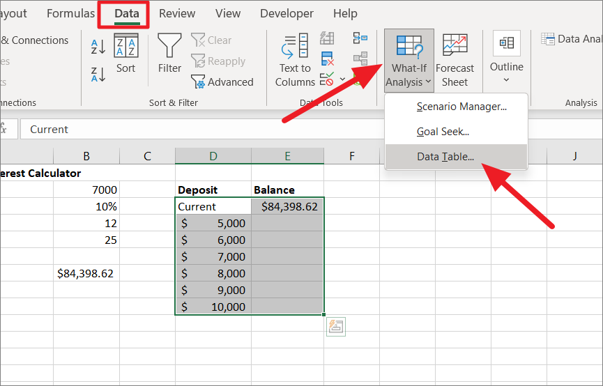
When the Data Table dialog pops up, click in the ‘Column input cell’ field, select the cell containing the initial investment value (for FV formula), and click ‘OK’. Here, we are selecting cell B2.

As soon as you click ‘OK’, Excel will populate the empty cell with results (final balances) corresponding to the variable values next to it.

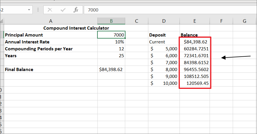
Now, you have the one-variable table with different initial deposits and their final balances after 25 years. Then, you can decide the optimal deposit amount for your investment with this data table.

You can also change the variables in the ‘Deposit’ column to further test the outcomes.

Calculate Compound Interest using Two Variable Data Table

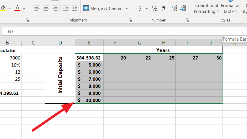
In the above example, we used What-if analysis to determine the right investment value. But what if you don’t know the correct deposit amount and how long you should have the interest compound to reach about $100,000? In that case, you should use a two-variable data table to calculate the future value of an investment based on different Initial deposits and the number of years.

A two-variable data table shows you how the results of a formula change based on two different sets of input variables. In other words, it allows you to analyze the effect of changing two input variables on the outcome of a calculation.

For this, we are going to use the same compound interest formula we used before to test how changes in the initial investment and the number of years values affect the balance:

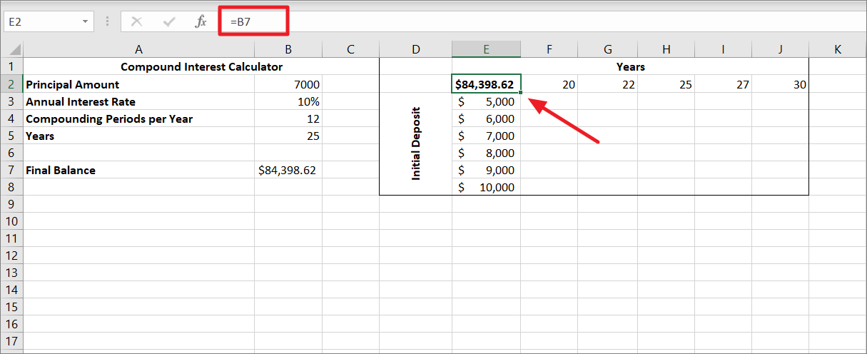
First, create a two-dimensional data table for two sets of variables. The top left corner cell should be the formula cell and it should be linked to your original formula cell. Here, we are linking cell E2 to the compound interest formula cell B7 with =B7.

Ensure there are enough empty columns to the right and empty rows below to fit variable values and the results.

Next, enter one set of variable values (either initial deposit amounts or the number of years) right below the formula (E2) in the same column. And type the other set of input values to the right of the formula, in the same row. In this example, we typed initial deposits in E3:E9 and the years in F2:J2.

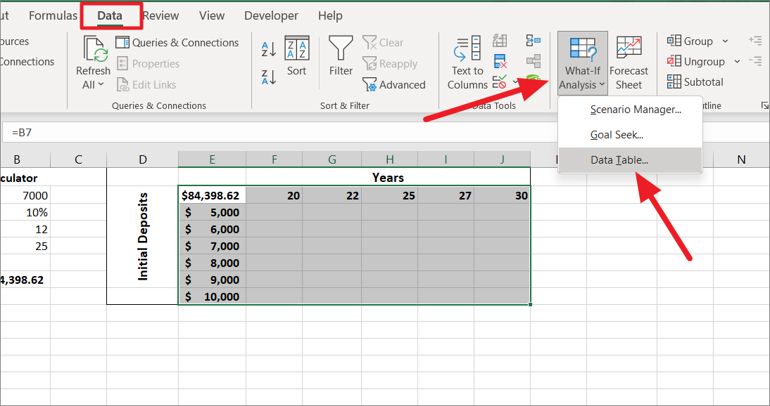
After that, select the entire data table range containing your formula, input values cells, and empty cells for the results. Here, we selected the range D1:J9.

Then, switch to the ‘Data’ tab, click the ‘What-If Analysis’ button in the Forecast group, and select ‘Data Table..’ from the menu.

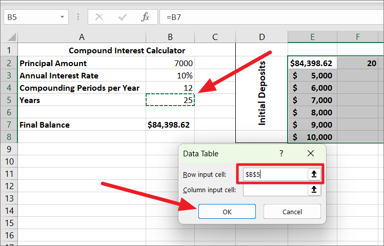
In the Data Table dialog box, click in the ‘Row input cell’ field, and select the cell containing the Years value (B5).

Then, click in the ‘Column input cell’ field, select the cell with initial investment value (B2), and click ‘OK’.

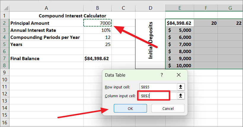
Once, you click ‘OK’, Excel will immediately populate the results cells in the data table. Now, you can see the effects of two different sets of variables on the FV formula’s result.

How to Calculate the Compound Annual Growth Rate (CAGR) in Excel

So far we learned how to calculate Compound Interest in several ways. We will take it one step further and see how to calculate the Compound Annual Growth Rate (CAGR) in Excel. Compound Interest and Compound Annual Growth Rate (CAGR) are related in that both are used to measure growth over time. However, they measure growth in different ways.

The Compound Annual Growth Rate (CAGR) is a financial metric that represents the average rate of return of an investment over a specified time period, assuming the investment compounds over time. It’s used to calculate the average growth rate of an investment or portfolio over a specified period, such as years.

The Compound Annual Growth Rate (CAGR) is very helpful for business, financial planning, financial modeling, and investment analysis. To calculate CAGR you need three primary inputs: an investment’s starting value, ending value, and the number of periods (years).

CAGR Formula

The syntax of the CARG formula is:

CAGR =(Ending value/Beginning value)1/n - 1

where:

Ending value – Ending the balance of the investment at the end of the investment period.
Beginning value – The beginning balance of the investment at the start of the investment period.
n – Number of years you have invested.

Calculating CAGR in Excel Using Operators

The direct way to calculate CAGR is by using operators. Use the above generic formula to calculate CAGR.

Let’s assume we have sales data for a certain company in the spreadsheet below.

Column A has the years in which the revenues are earned. Column B has the revenue of the company in the respective year. With the CAGR formula in excel, you can calculate the annual growth rate for the revenue.

Enter the below formula to calculate CAGR by the direct method:

=(B11/B2)^(1/9)-1

In the example below, the investment’s starting value is in cell B2 and the ending value is in cell B11. The number of years (period) between the start and the end of the investment period is 9. Usually, each investment cycle period starts one year and ends the next year, hence, the first period of the cycle, in this case, is 2011-2012 and the last cycle is 2019-2020. So the total number of years invested is ‘9’

The result will be in decimal numbers not in percentages as shown above. To convert it to a percentage, go to the ‘Home’ tab, click on the drop-down that says ‘General’ in the Number group, and select the ‘% Percentage’ option.

Now, we got a compound annual growth rate that is ‘11.25%’ in cell B13. This is the single smoothed growth rate for the whole time period.

Calculating CAGR in Excel Using POWER Function

Another easy method to calculate Compounded annual growth rate (CAGR) in Excel is by using the POWER function. The POWER function replaces the ^ operator in the CAGR function.

The syntax of the POWER function:

=POWER(number,power)

Arguments of the POWER function:

number – It is the base number found by dividing the ending value (EV) by the beginning value (BV) (EV/BV).
power – It is to raise the result to an exponent of one divided by duration (1/number of periods (n)).

Now, the arguments are defined this way to find the CAGR value:

=POWER(EV/BV,1/n)-1

Let’s apply the formula to an example:

=POWER(C11/C2,1/A11)-1

The result:

Calculating CAGR in Excel Using the RATE Function

The RATE function is yet another function you can use to find CAGR in Excel. When you look at the syntax of the RATE function, it may look a bit complicated with 6 arguments no less, but once understand the function, you may prefer this method for finding the CAGR value.

The Syntax of the RATE function:

=RATE(nper,pmt,pv,[fv],[type],[guess])

Where:

nper – The total number of payments period (the loan term).
Pmt (optional) – The amount of the payment made in each period.
pv – This specifies the present value of the loan/investment (beginning value (BV))
[fv] – This specifies the future value of the loan/investment, at the last payment (ending value (EV))
[type] – This specifies when the payments for the loan/investment are due, it is either 0 or 1. The argument 0 means the payments are due at the start of the period and 1 means payments are due at the end of the period (default is 0).
[guess] – Your guess of rate. If omitted, it defaults to 10%.

The reason the RATE function has six arguments is that it can be used for many other financial calculations. But we can convert the RATE function to a CAGR formula, with only three arguments 1st (nper), 3rd (pv), and 4th (fv) arguments:

=RATE(nper,,-BV,EV)

Since we don’t make regular payments (monthly, quarterly, yearly), we leave the second argument empty.

To calculate the compound annual growth rate using the RATE function, use this formula:

=RATE(A11,,-C2,C11)

If you don’t want to calculate the number of periods manually, use the ROW function as the first argument of the RATE formula. It will compute the npr for you.