
When you’re working with data in Excel, you may need to compare columns to find similarities and differences between data. Comparing columns is very useful for organizing and analyzing data. Manually comparing the data from two columns can be a time-consuming and exhausting task, so you can use various Excel formulas to match columns.
Excel has several methods and functions for comparing columns and finding matching and mismatching data. You can use logical operators – VLOOKUP, MATCH, AND, INDEX, IF, COUNTIF, ISERROR, IFERROR – or Conditional Formatting rules to compare and match data. In this article, we will discuss different methods to compare columns in Excel for matches and differences.
Comparing Two Columns Row by Row for Matches or Differences
The simplest way to compare two columns in Excel is a simple row-by-row, line-by-line comparison. This method checks whether the value in one column matches the value in another column in the same row. It will only compare values in the same row, not the entire dataset. There are different types of formulas you can use to compare two columns row by row – using a simple comparison operator, IF function, and EXACT function.
Compare Columns Using Equals Operator
The easiest way to compare two columns’ data row by row for finding the match is using the comparison operator. With the ‘Equals to’ (=), you can compare cells in two columns for a match and get the result as either true or false.
Example 1:
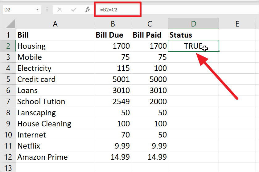
For example, we will compare two columns (Bill Due and Bill Paid in the screenshot below) to see if they match. To do that, we will use the below simple formula:
=B2=C2The value in B2 matches the value in C2, so the formula returns TRUE. First, enter the formula in cell D2 and then copy it down to other cells by dragging the fill handle to compare columns B and C row by row. The fill handle is a small green square in the bottom right corner of the selected cell.
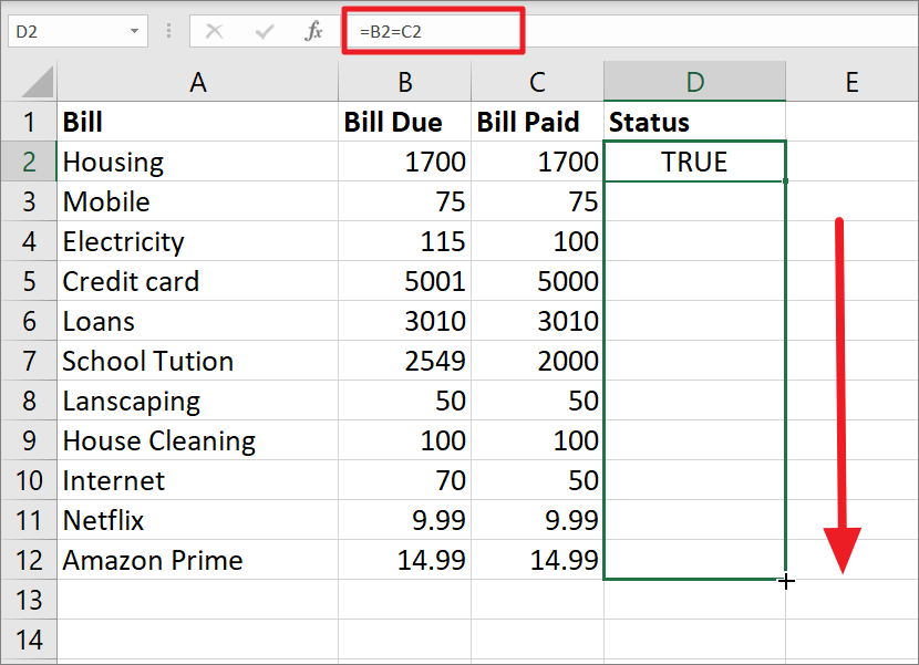
When you drag the fill handle from cell D2 to D12, the cursor will change into a black plus sign.
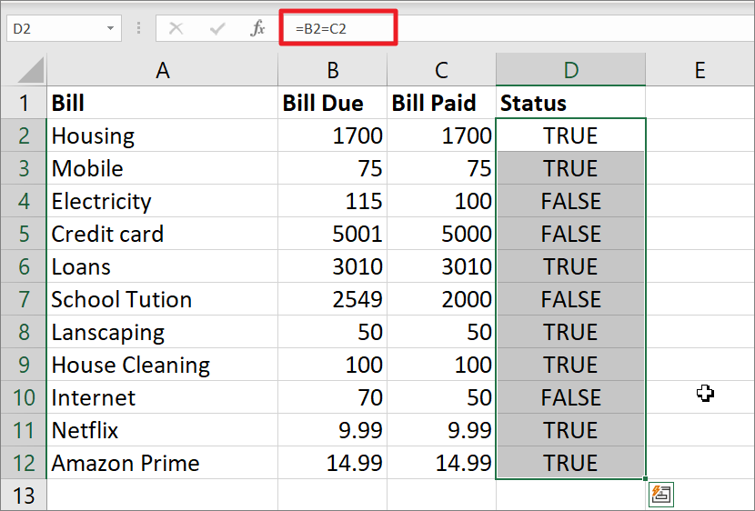
As you apply the formula through cells D2 to D12, it will compare values row by row and you will see some rows matches while others don’t. For example, the value from cell B4 does not match its adjacent cell C4, hence the value in cell D4 is FALSE.
Example 2:
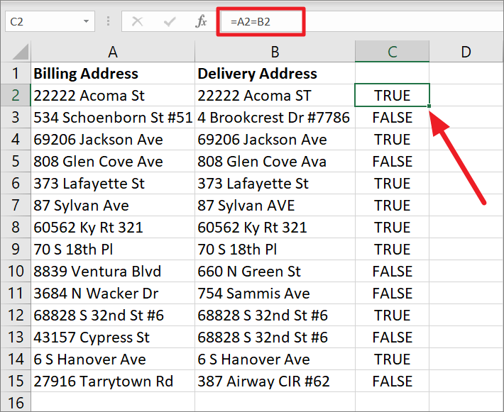
We have seen how the above formula handles numbers, but it can also compare dates, times, and text strings equally well. Let us see how the formula compares columns with text values.
=A2=B2The formula looks for the correct match between the two columns and will not miss even a single space character. Then it returns TRUE if the condition is met or else returns FALSE. The billing address in cell A2 matches the delivery address in cell B2, as a result, we get TRUE. Also, the address in cell A5 does not match the address in cell B5 – the last character is different in cell B5. Hence, it returns FALSE.
Compare Columns using IF Function
Another way we can compare two columns row by row is by using the IF function. The IF function checks whether a condition or criteria is met and returns one specified value if the condition is TRUE or another value if the condition is FALSE. Although this method is similar to the above method, we can use it to get more descriptive results than just TRUE or FALSE.
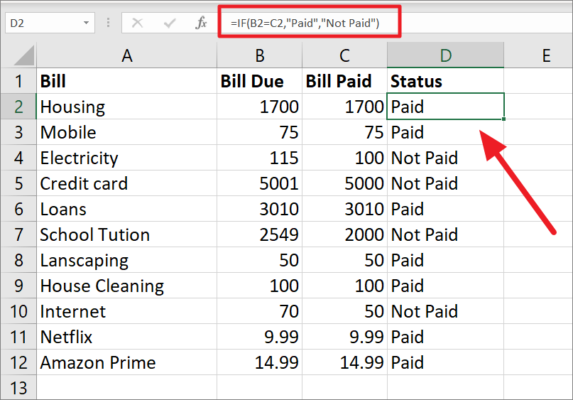
For example, we can use the below formula to compare two columns and if there is a match, we can get the result “Paid” or “Not Paid” if there is no match:
=IF(B2=C2,"Paid","Not Paid")In the above formula, the IF function checks if the value in B2 is equal to the value in C2, and if the condition is True, it returns the text “Paid”. If the condition is False, it returns “Not Paid”. The Bill due amount in B2 and Bill Paid amount in C2 are the same, so it returns “Paid” in D2. But the amount in B5 and C5 do not match, so the formula returns “Not Paid” in D5.
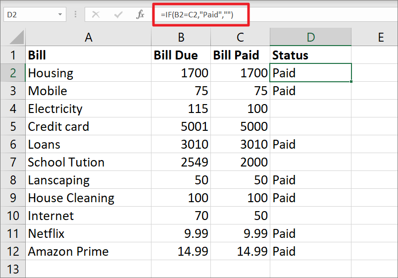
For Matches Only:
In case you want to find only matches in two columns, you can use the below formula:
=IF(B2=C2,"Paid","")The above formula checks if the value in column B is equal to the values in column C, row by row. If the condition is true, we will get the “Paid” text string and if the condition is false, we will get nothing (empty string).
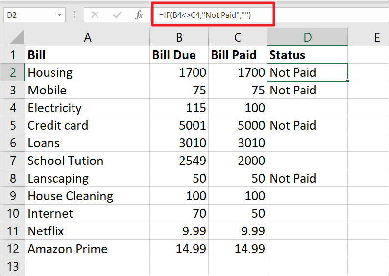
For Difference Only:
To find cells with different values in the same row, try the below formula:
=IF(B4<>C4,"Not Paid","")The above formula checks if the values in column B are not equal to the values in column C, row by row. If the condition is true, we will get the “Not Paid” text string and if the condition is false, we will get nothing (empty string).
Note: The equals to formula and IF function formulas are case-insensitive which means they will ignore cases when comparing text values.
Compare Two Columns for Case-Sensitive Match in the Same Row using the EXACT function
The above formulas ignore cases when comparing text values. If you want to make the comparison case-sensitive, you need to use the EXACT function. The Excel EXACT function is used to compare two text strings and returns TRUE if both values are the same, and FALSE otherwise. You can either use EXACT alone or with the IF function (in case you want to get a descriptive result instead of just TRUE or FALSE.
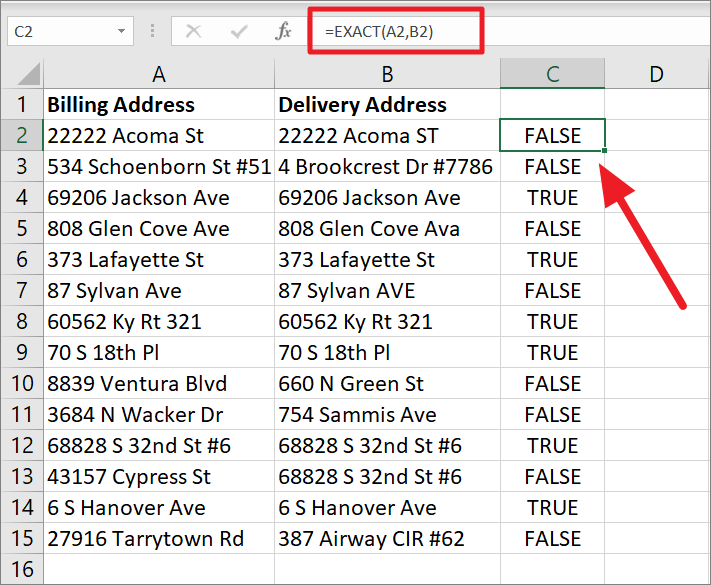
For example, let’s compare lists of company names from different databases and see if they are exact matches using the simple EXACT function:
=EXACT(A2,B2)The above formula checks if the text strings from A2 and B2 are an exact case-sensitive match. Then, it returns FALSE because the word “St” in A2 is in lowercase while in B2, it is capitalized.
In case you want to get descriptive results, you need to use the IF function with the EXACT function:
=IF(EXACT(A3,B3),"Match", "Check Database")In the above formula, the EXACT function checks whether the values in cells A3 and B3 are exact case-sensitive matches or not. However, the first-word ‘ANGELO’ is capitalized in B2 which is different from the company name in A2, so the EXACT function returns FALSE. Hence, the IF function returns the “Check Database” text string for the FALSE output.
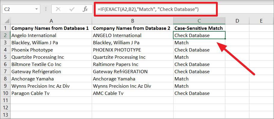
In row 5, cell values A5 and B5 are case-sensitive matches, so the IF function gets a TRUE result from the EXACT function and returns “MATCH” in its place.
Compare Two Columns If Greater Than Or Less Than
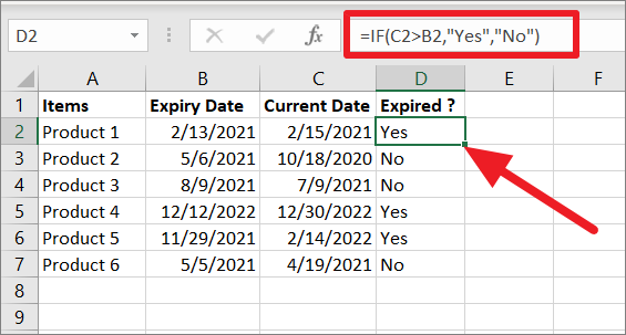
Sometimes, you may want to compare columns and check if the values in one column are greater or less than the other columns. For example, if you have two columns of dates and you want to compare which date is later in the same row (perhaps to compare the expiry date of products), you can use a simple logical operation to find out.
To find out if the products are expired or not, compare two columns if column C is greater than column B:
=IF(C2>B2,"Yes","No")The above formula checks if the value in cell C2 is greater than cell B2. If it is TRUE, then the IF function returns ‘Yes’, otherwise ‘No’.
Compare Multiple Columns Row by Row for Matches
We have seen how to compare two columns row by row but you can also compare multiple columns for matches in the same row. There are two ways you can compare multiple columns – find matches within all cells in the same row or find matches in any two cells in the same row.
Find Matches in All Cells Within the Same Row
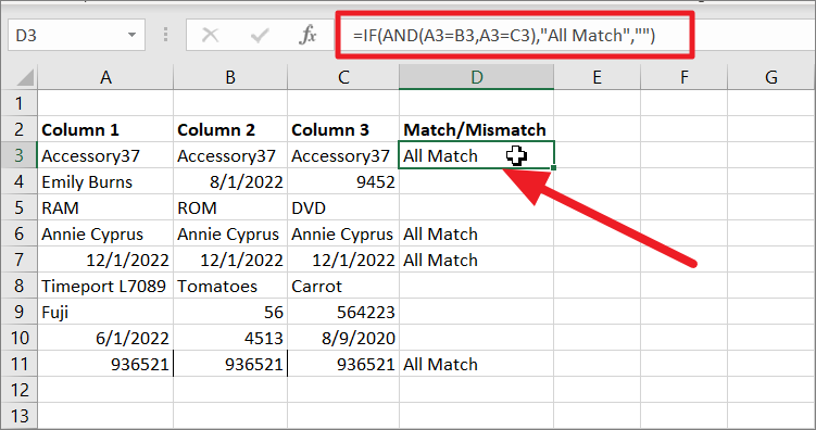
Method 1: If you have a dataset with more than two columns (multiple columns) and you want to find rows with the same values in all columns. You can do this with IF and AND functions:
=IF(AND(A3=B3,A3=C3),"All Match","")The AND function tests multiple conditions at the same (A3=B3 and A3=C3) and returns TRUE only if all its arguments evaluate to TRUE. AND function will return FALSE even if one of the arguments evaluates to FALSE. You can add multiple conditions in the AND function by including a comma between each condition.
As you can see below, the AND function will return true if all the cells have the same value in the same row. Then, the IF function will return the text “All Match” if the AND function returns TRUE.
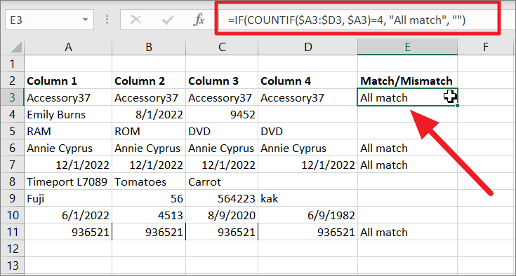
Method 2: If your dataset has a lot of columns, you can use the COUNTIF function to make your formula compact:
=IF(COUNTIF($A3:$D3, $A3)=4, "All match", "")Where 4 represents the number of columns you are comparing in the formula. The COUNTIF function is used to count the numbers that meet a specific single criterion.
The COUNTIF formula checks whether the row has the same values in all cells (A3:D3), and returns the total number of matches. And if all the columns match within the same row (the result of the COUNTIF function) is equal to the number of columns, you will get the text string that says “All match”.
Find Matches in Any Two Cells in the Same Row
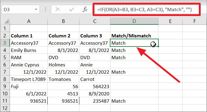
Method 1: Suppose you have multiple (3) columns and you want to find matches in any of the two columns in the same row, you can do that with the help of the IF and OR functions. To do this, we can use the below formula:
=IF(OR(A3=B3, B3=C3, A3=C3), "Match", "")In the above formula, OR function compares each column against other columns and if any of the two or more columns with the same value match within the same row, it will return TRUE. The IF function will return the text ‘Match’ when it gets TRUE from the OR function.
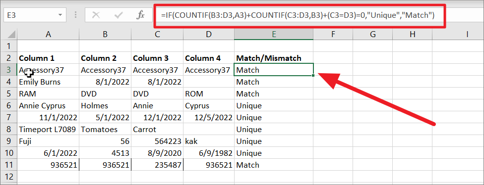
Method 2: If you have too many columns to compare, the above OR formula can get too big and complicated. To avoid this, you can add up several COUNTIF functions:
=IF(COUNTIF(B3:D3,A3)+COUNTIF(C3:D3,B3)+(C3=D3)=0,"Unique","Match")Here, the first COUNTIF function checks and counts how many cells (columns) have the same value as the first column (A3), and the second COUNTIF function checks how many columns have the same values as the second column, and so on. Then all the COUNTIF function results are added up. So, if the final count is equal to 0, the formula will return the ‘Unique’ text string. If the count is anything other than 0, we will get ‘Match’ as the result.
Compare and Highlight Matching/Mismatching Columns
If you want to compare two columns and highlight the rows that have matching data or mismatching data instead of showing the result in a separate column, you can use conditional formatting in Excel. Conditional formatting is a feature in Excel that can highlight data based on a set of rules. With conditional formatting, you can visually identify matching values or different values in two columns.
Compare Two Columns and Highlight Matching Data in the Same Row (Side by Side)
If you want to compare two columns and highlight the identical data in the same rows, follow the below steps:
First, select the cells you want to compare and highlight. You can either choose a single column or multiple columns if you want to highlight entire rows.
Under the ‘Home’ tab, click the ‘Conditional Formatting’ menu in the Styles group and select the ‘New Rule…’ option from the menu.
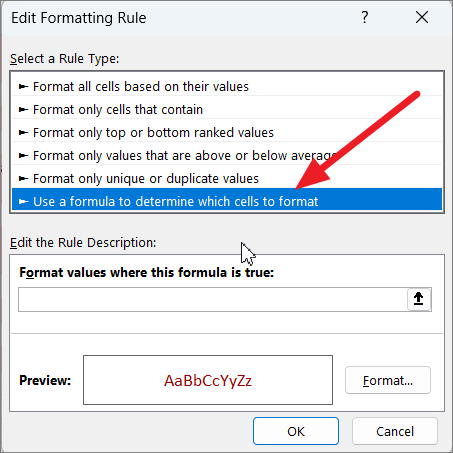
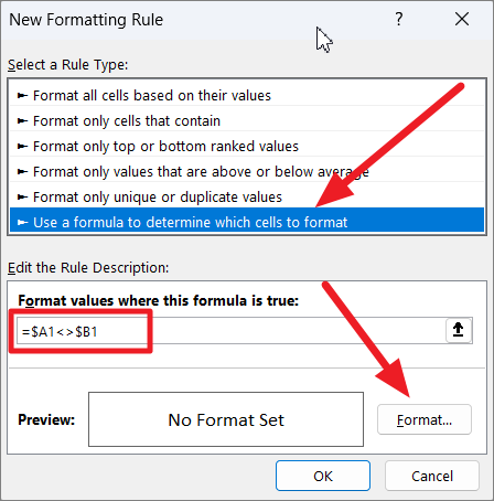
This will open the New Formatting Rule dialog box. In that dialog window, select the rule type ‘Use a formula to determine which cells to format’.
After that, type the following formula in the ‘Format values where this formula is true:’ field:
=$A1=$B1As you can see, this is a simple ‘equals to’ formula that checks whether the value in cell A1 is equal to B1. But we have added the ‘$’ sign before the column labels A and B to lock the columns into absolute references. So, only the row number automatically changes for each row when the formula is applied.
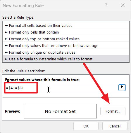
Next, click on the ‘Format’ button to customize the look you want for the highlighted rows.
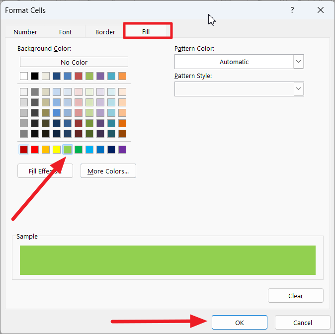
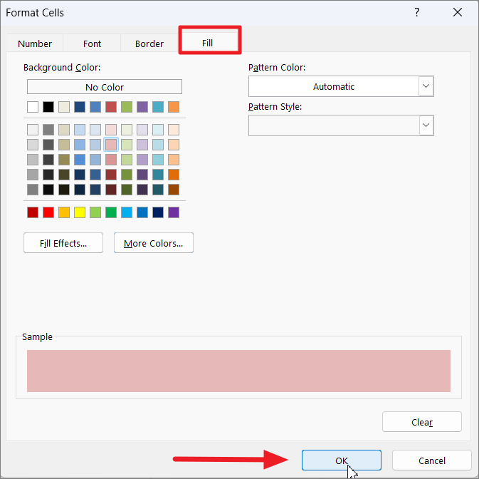
In the Format cells dialog window, you can change the font size, font color, cell borders, number format, etc. To highlight matching rows with different background colors, switch to the Fill tab and choose the color from the Background color section. You can also change the pattern style and pattern color of the highlighted cells. Once you are done choosing the format, click the ‘OK’ button.
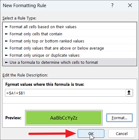
Again, click ‘OK’ in the New Formatting Rule dialog box to apply the formatting
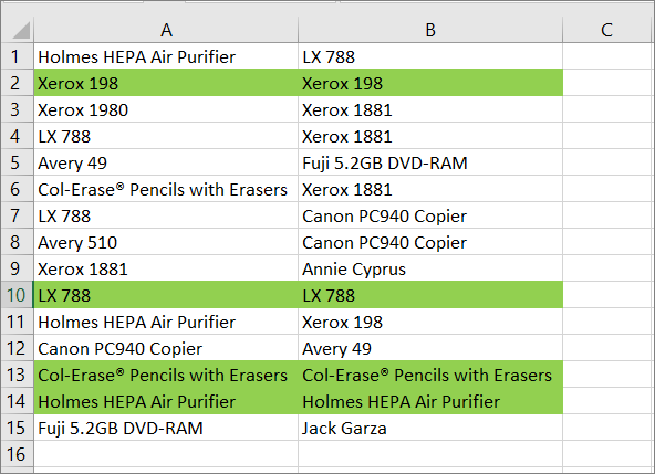
The cells with matching values in both columns A and B will be highlighted as shown below.
If you have fewer matching data than mismatching data in the table, you can flip the condition to highlight the data difference between the two columns.
For instance, we can use either of the below conditional formatting rules to highlight the difference between columns A and B:
=$A1<>$B1or
=$A1=$B1=FALSEFirst, select the dataset and open the New formatting rule window, as we showed you above, and then select the ‘Use a formula to determine which cells to format’ rule type. Then, enter one of the above rules and click the ‘Format’ button.
Next, choose the formatting you want to apply and click ‘OK’. And click ‘OK’ again to apply the formatting.
Compare Two Columns and Highlight Duplicate Values
If you want to compare two columns and highlight the values existing in both columns even when they’re not in the same row, you can use the preset Conditional Formatting rules or custom formatting rules.
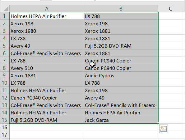
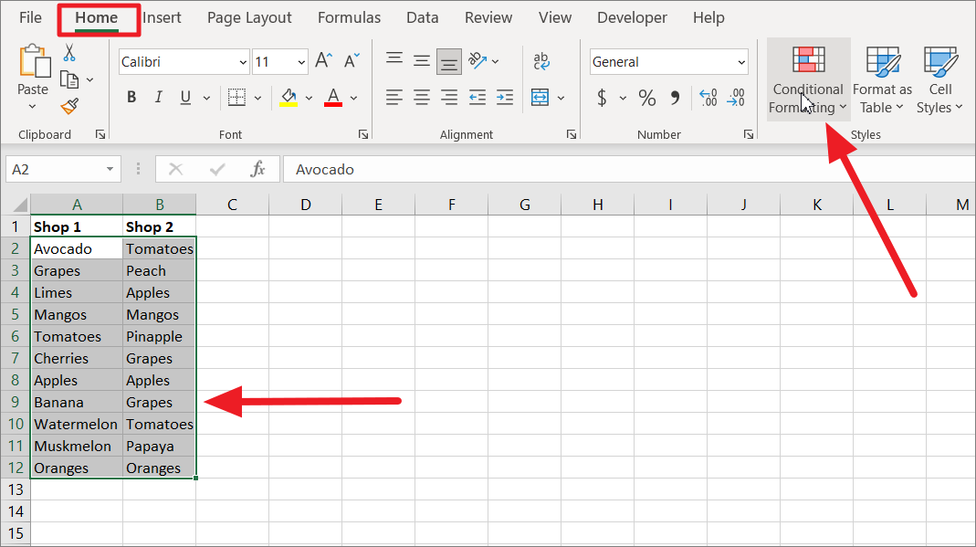
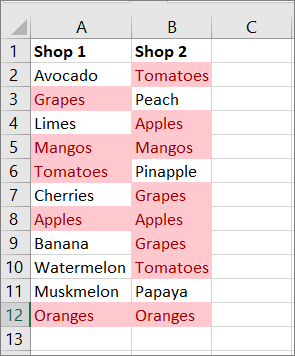
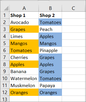
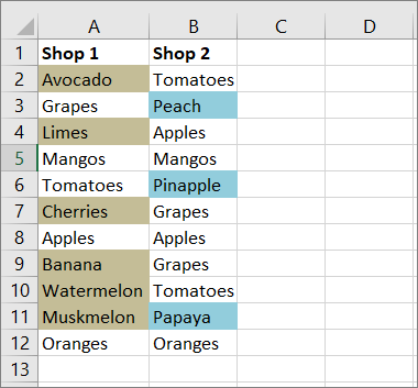
For instance, we have two lists of fruits from different shops and we want to highlight the fruits that are available at both shops. Here’s how you can do that:
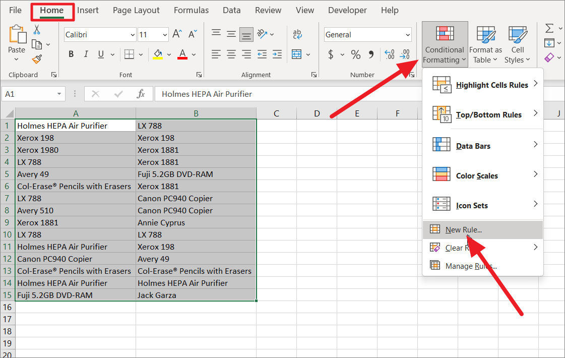
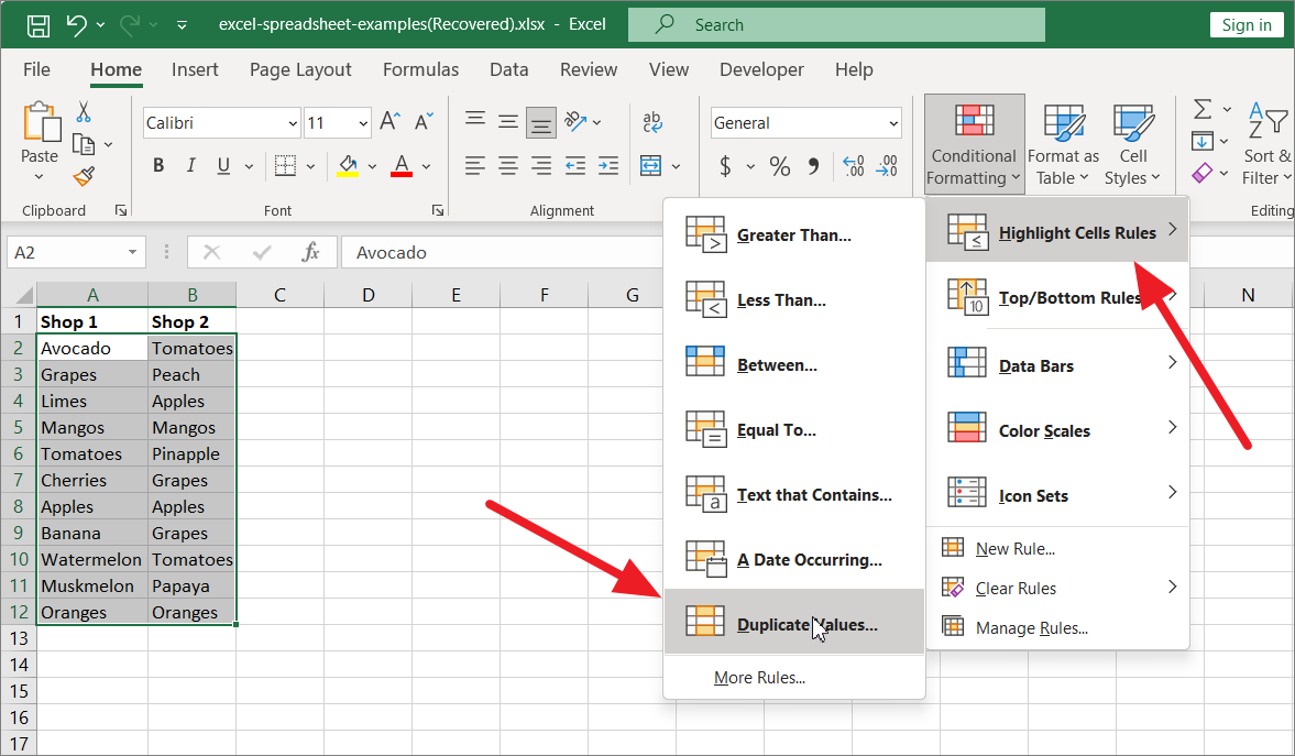
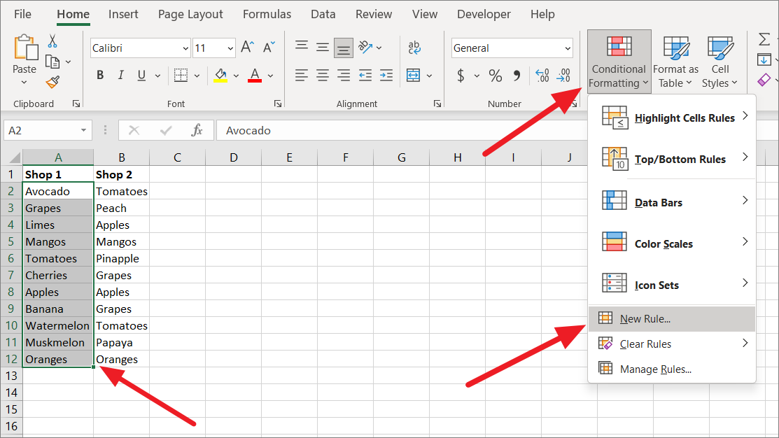
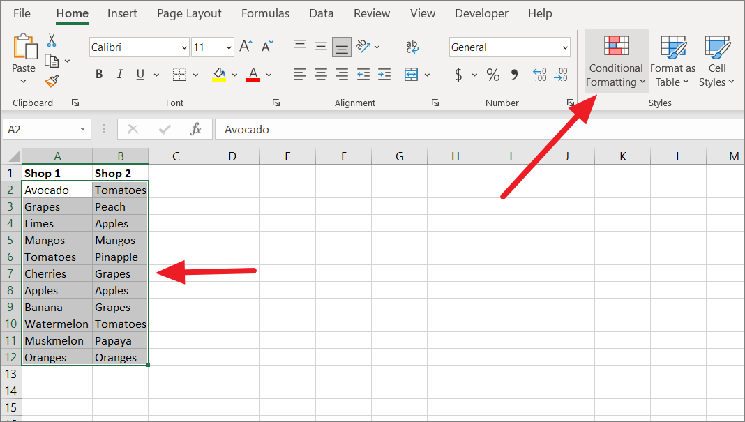
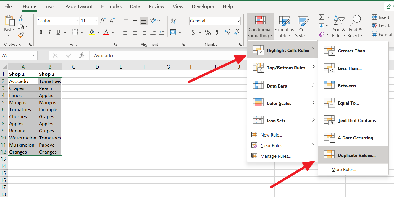
First, select the columns you want to compare and click the ‘Conditional Formatting’ menu from the Styles group.
Then, hover the cursor on the ‘Highlight Cell Rules’ option from the drop-down menu and select the ‘Duplicate Values’ option.
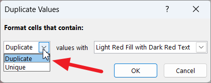
In the Duplicate Values dialog box, select ‘Duplicate’ from the left side drop-down.
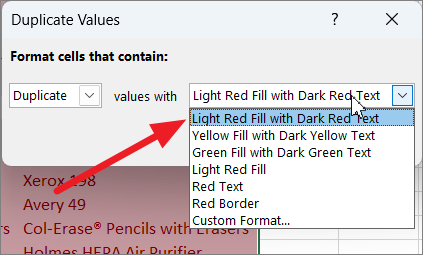
Then, select the format from the right-side drop-down menu and click ‘OK’.
The items that exist on both columns will be highlighted.
Alternatively, you can also use custom formatting rules to highlight duplicate values in two columns.
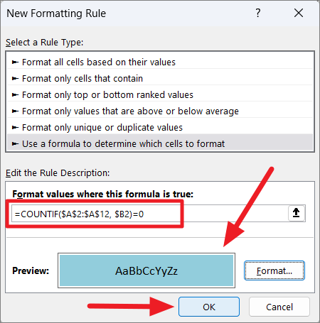
To do that, first, select column A and click the ‘Conditional Formatting’ option from the ribbon. Then, select the ‘New Rule’ option from the menu.
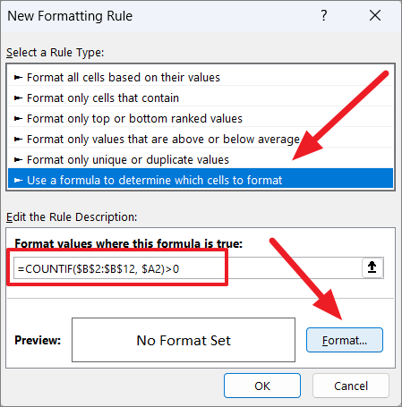
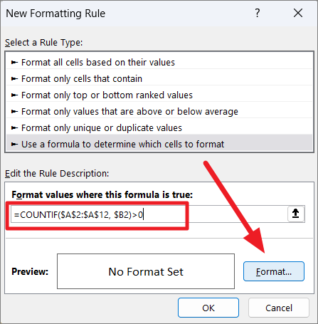
After that, select the ‘Use a formula to determine which cells to format’ rule type and enter the below rule to highlight the matches in column A:
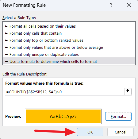
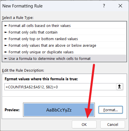
=COUNTIF($B$2:$B$12, $A2)>0Then, click the ‘Format’ button to select the formatting you want to apply and apply those.
Click ‘Ok’ to apply the formatting to column A.
Next, select column B and click the ‘Conditional Formatting’ option from the ribbon. Then, select the ‘New Rule’ option from the menu.
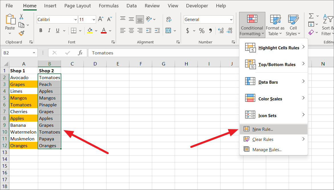
In the New Formatting Rule window, choose the ‘Use a formula to determine which cells to format’ rule type and enter the below to highlight duplicates in column B:
=COUNTIF($A$2:$A$12, $B2)>0After entering the formula, click the ‘Format’ button and specify the formatting for highlighting cells.
After choosing the format, click ‘OK’ to apply it.
Now, duplicate values in both columns have been highlighted.
Compare Two Columns and Highlight Unique Values
This method is the exact opposite of the above method. If you want to compare two columns and highlight only unique values in both columns that do not match, you can use conditional formatting for this too.
First, select the columns you want to compare, go to the ‘Home’ tab, and then click the ‘Conditional Formatting’ menu in the Styles group.
Then, hover over the ‘Highlight Cell Rules’ options and select ‘Duplicate Values’.
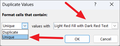
In the drop menu that says Duplicate, select ‘Unique’ and then choose predefined formatting for the mismatched data. Then, click ‘OK’.
Now, the unique or mismatched values from both columns are highlighted.
Alternatively, you can also use custom formatting rules to highlight unique values in two columns.
To do that, first, select column A and click the ‘Conditional Formatting’ option from the ribbon. Then, select the ‘New Rule’ option from the menu.
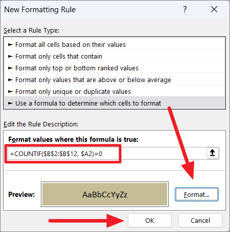
After that, select ‘Use a formula to determine which cells to format’ rule type and enter the below rule to highlight the matches in column A:
=COUNTIF($B$2:$B$12, $A2)=0Then, click the ‘Format’ button to choose formatting.
Click ‘Ok’ to apply the formatting to column A.
Next, select column B and click the ‘Conditional Formatting’ option from the ribbon. Then, select the ‘New Rule’ option from the menu.
In the New Formatting Rule window, choose the ‘Use a formula to determine which cells to format’ rule type and enter the below to highlight duplicates in column B:
=COUNTIF($A$2:$A$12, $B2)=0After entering the formula, click the ‘Format’ button and specify the formatting for highlighting cells. Then, click ‘OK’ to apply it.
Now, unique values in both columns have been highlighted.
Compare Multiple Columns and Highlight Matching Rows
We have seen how to compare two columns and highlight row matches but if you have multiple columns that need to be compared, you can also do that with the help of conditional formatting. With conditional formatting, we can compare several columns, row by row, and highlight the matches.
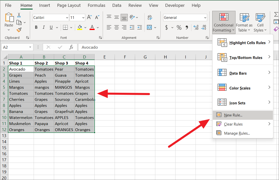
For instance, we have lists of fruits from three different shops and we want to highlight the rows that have identical items in all three columns. To do that, follow these steps:
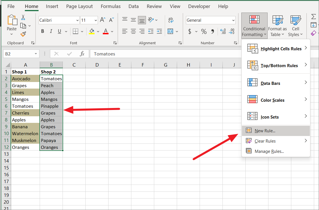
First, select the columns for comparison (A2:D12). Then, click the ‘Conditional Formatting’ menu and select the ‘New Rule..’ option.
To compare multiple columns, create a new conditional formatting rule with the AND or COUNTIF function:
=AND($A2=$B2, $A2=$C2, $A2=$D2)Where columns A, B, and C are locked into absolute references using the $ sign while row number (2) is left as a relative reference. So the formula can automatically change to compare values row by row. When the above formula is applied to the table, it compares the first row of the table. Then, the formula automatically adjusts itself to =AND($A3=$B3, $A3=$C3, $A3=$D3), and so on. Only the row numbers changes since they are relative references and the column letters remain the same because they are absolute references.
Each cell value in the row is compared against the value of the first column. When all the conditions are satisfied, the AND function returns TRUE. If the result of the conditional formatting rule is TRUE, then the respective row is highlighted with the specified formatting.
In the New Formatting Rule window, select ‘Use a formula to determine which cells to format’ and type the above formula in the ‘Format values where this formula is true:’ text field. Then, click ‘Format’ to specify formatting.

After selecting the formatting, click ‘Ok’ to apply the conditional formatting.

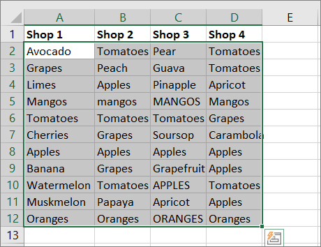
Now, the rows with the same values in multiple columns are highlighted.

In case you have a lot of columns to compare, you can also use the COUNTIF function to create a conditional formatting rule:
=COUNTIF($A2:$D2, $A2)=4Where A2 will be compared against every cell in the first row (A2:D2) and 4 is the number of columns to compare. The formula checks whether A2 matches with other cells in the row. If the row has identical values in all four columns, the COUNTIF function would return 4. If the COUNTIF function result is equal to the number of columns (4), the Conditional formatting rule would result in TRUE and the respective row will be highlighted.
The above conditional formatting rule will automatically adjust itself to compare each row in the table.
To start with, select the columns for comparison, click the ‘Conditional Formatting’ menu and select ‘New Rule…’

Next, select the ‘Use a formula to determine which cells to format’ rule type and enter the above formula in the text field below. After that, specify the formatting for the highlights and click ‘OK’.

Now, the rows with the same values in multiple columns are highlighted.

You should know that AND and COUNTIF formulas can be used to compare more than 4 columns and highlight rows with the same values.
Compare Multiple Columns and Highlight Row Differences
If you want to compare multiple columns and highlight different values (mismatched data) in each individual row, you can use the ‘Go To Special’ feature in Excel.
To do this, select the columns you want to compare.
Now, you need to specify the comparison column. Cell values from other selected columns from the same row will be compared against the comparison column to highlight the cell difference. When you select a range, the top cell of the range is the active cell. In the above image, the active cell is white while other cells are grey highlighted. Here, the active cell is A3, hence the comparison column is A.
To change the comparison column, press the Tab key to move the active cell from left to right or hit Enter key to move from top to bottom.
Then, click the ‘Find & Select’ menu button from the ‘Editing’ group of the ‘Home’ tab and select ‘Go To Special…’.
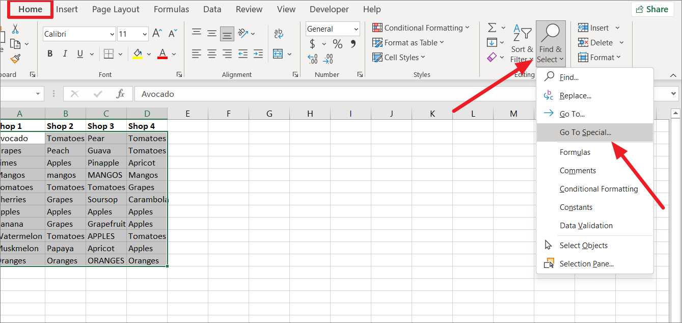
In the Go To Special dialog box, select ‘Row differences’ and click the ‘OK’ button.

As you can see, all the cell values that are different in the comparison column in each row will be highlighted/selected.

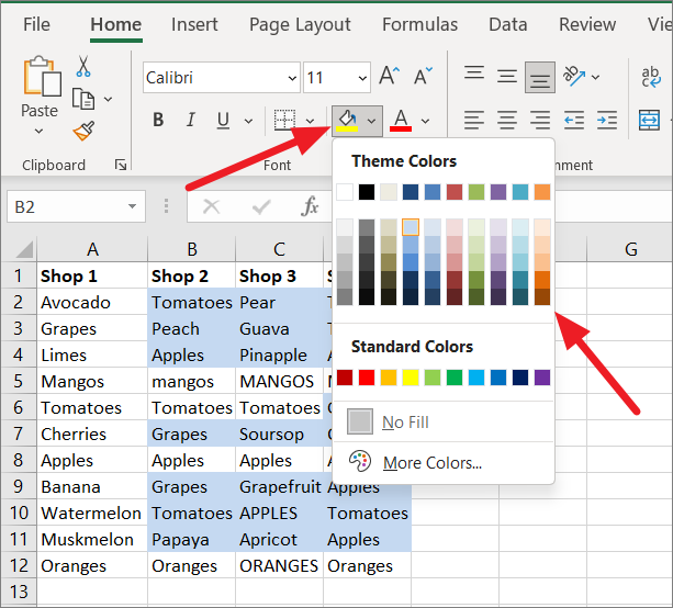
To highlight the selected cells with a color, click the ‘Fill Color’ button on the ribbon and pick a color from the palette.
Compare Two Columns Using VLOOKUP and Extract Matching Data
Sometimes, you may not only want to compare items in one list to the other, but also pull matching data. When comparing columns, there are two types of matches you can use – a partial match or an exact match. This can be done with VLOOKUP or INDEX MATCH function.
The VLOOKUP function is used to search for a specific value in a column and returns a corresponding value from a different column in the same row.
Syntax of VLOOKUP function:
=VLOOKUP(lookup_value,table_array,col_index_num,[range_lookup])This function consists of 4 parameters or arguments:
- lookup_value: This specifies the value that you are searching for in the first column of the given table array. The Lookup value must always be in the left-most column of the search table.
- table_array: This is the table (range of cells) in which you want to look up a value. This table (search table) can be in the same worksheet or different worksheet, or even a different workbook.
- col_index_num: This specifies the column number of the table array that has the value you wish to extract.
- [range_lookup]: This parameter specifies if you want to extract an exact match or an approximate match. It’s either TRUE or FALSE, enter ‘FALSE’ if you want the exact value or enter ‘TRUE’ if you’re OK with the approximate value.
Exact Match
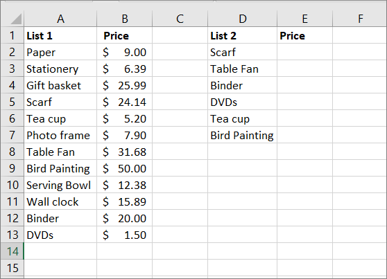
Let’s assume we have two tables with a list of items. In the second, we have a list of items and their prices need to be filled. To do that, we need to compare column A with column D and extract prices for the matching items.
We can use the VLOOKUP function to compare two columns and fetch matching data:
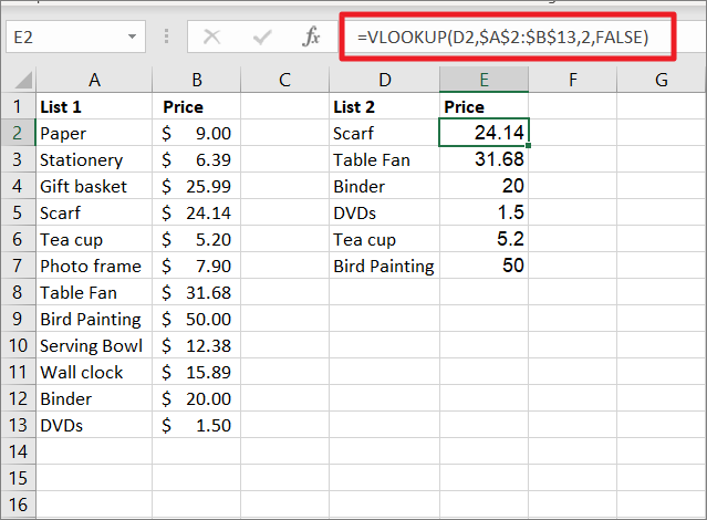
=VLOOKUP(D2,$A$2:$B$13,2,FALSE)
First, enter the formula in cell E2 and then copy the formula down the column by dragging the fill handle.
Where D2 is the value that needs to be searched in the first column of the lookup table. $A$2:$B$13 represents the lookup table where the value will be searched and the corresponding value will be pulled. Here the range is locked into absolute references to prevent the cell reference from changing as the formula is copied down.
The ‘2’ in the formula is the column number of the lookup table with the value you wish to extract. The FALSE parameter is used to find the exact match of D2.
The above formula will search the first column of the range A2:B13 (column A) for the value in D2. An exact match of D2 is found in row 5 of column A, so the corresponding value is extracted from column B (column 2) and returned in E2. When the formula is copied down column E, only the lookup_value value automatically adjusts to D3, D4, etc to search each value of column D in the range A2:B13.
Compare Columns and Pull Matching Data using IFERROR or IFNA functions
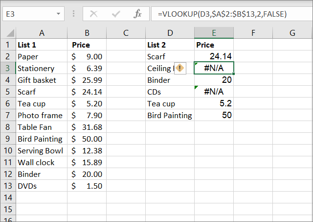
In case the lookup_value is not found in the lookup table or the look_up value weren’t exact copies of the values in the look_up table, you would get the #N/A error.
In the below example, lookup_values (D3 and D5) weren’t found in column A and the match type is FALSE (exact), so the formula returns the #N/A error.
This can happen even if there is an extra space, missing space, or a typo in the look_up value. In such cases, you can change the match_type to TRUE which will enable the formula to ignore small errors and look for an approximate match of the values.
If the lookup_value is not found in the table, you can use IFNA or IFERROR function to avoid the #N/A error.
=IFNA(VLOOKUP(D2,$A$2:$B$13,2,FALSE),"")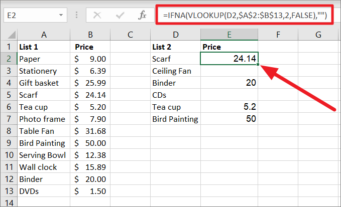
This formula works the same way as the previous VLOOKUP formula, except the IFNA replaces the error message with a blank. You can also have the formula return a text instead of a blank cell.
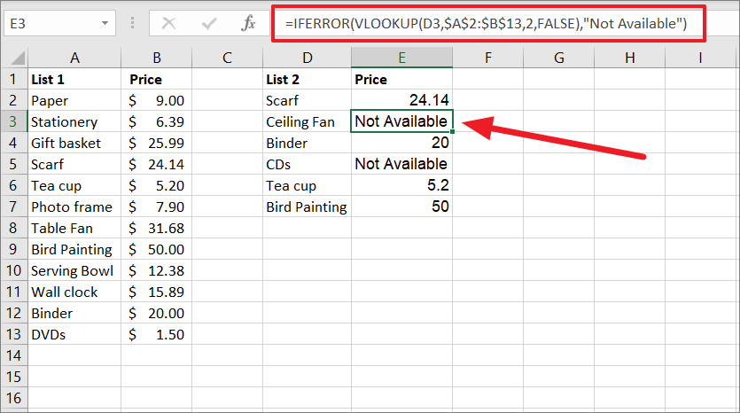
Alternatively, you can also use the IFERROR function to remove the error message and return a specified text string. To do that, enter the below formula:
=IFERROR(VLOOKUP(D2,$A$2:$B$13,2,FALSE),"Not Available")Enter the above formula in cell E2 and copy it down the column. If the VLOOKUP function returns an #N/A error, then the IFERROR function replaces it with the “Not Available” message as shown below.
Compare Two Columns and Find a Partial Match using Wildcards
In case there are minor differences in the names in the two columns, the TRUE parameter in the VLOOKUP function won’t cover it. For example, if one column has a value called “Google” and the other has “Google LLC”, the above VLOOKUP formula won’t be able to match the columns. However, you can still use the VLOOKUP to partially match columns by adding wildcards to the formula.
The VLOOKUP function allows you to find a partial match on a specified value using wildcard characters. If you want to locate a value that contains the lookup value in any position, add an ampersand sign (&) to join the lookup value with the wildcard character (*). Use ‘$’ signs to make absolute cell references and add the wildcard ‘*’ sign before or after the lookup value.
In the below example, we only have part of a lookup value (Fan) in cell D3. So, to perform a partial match on the given characters, concatenate a wildcard ‘*’ before and after the cell reference.
=VLOOKUP("*"&D3&"*",$A$2:$B$13,2,FALSE)In the above formula, D2 has been enclosed in ‘&’ operators and asterisks “*” to make up for the missing character before and after the lookup value. If List 2 doesn’t have the entire name of the items, the asterisks characters will make up for the missing characters and pull values from the partially matched columns.
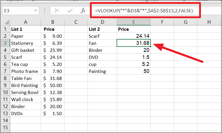
For instance, in cell D3 we only have the item named ‘Fan’ but in column A we have ‘Table Fan’. But the asterisks ‘*’ before the D3 made up for the missing ‘Table’ before the lookup value. So, the VLOOKUP function returns the corresponding value ‘31.68’ from column B.
Compare Two Columns using the MATCH Function
If you want to return the position of the matching value in the column instead of the value itself, you can use the MATCH function.
The MATCH function is a built-in function in Excel and its primarily used for locating the relative position of a lookup value in a column or a row.
Syntax of MATCH Function:
=MATCH(lookup_value,lookup_array,[match_type})Where:
lookup_value – The value you want to look up in a specified range of cells or an array. It can be a numeric value, text value, logical value, or a cell reference that has a value.
lookup_array – The arrays of cells in which you are searching for a value. It must be a single column or a single row.
match_type – It is an optional parameter that can be set to 0,1, or -1 and the default is 1.
- 0 looks for an exact match, and when it’s not found, returns an error.
- -1 looks for the smallest value that is greater than or equal to lookup_value when the lookup array is in ascending order.
- 1 looks for the largest value that is less than or equal to the look_up value when the lookup array is in descending order.
Compare Two Columns and Find the Position of An Exact Match
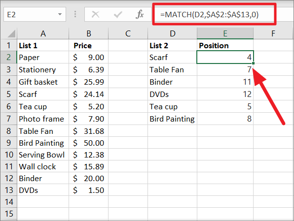
Let’s assume, we have the following tables where we want to find the position of each value in column D in column A.
=MATCH(D2,$A$2:$A$13,0)The formula searches for each value of list 2 in list 1 and returns the position of each value.
Display Duplicates or Matching Data using the MATCH function
A combination of MATCH, ISERROR, and IF functions can be used to compare and display duplicates of columns.
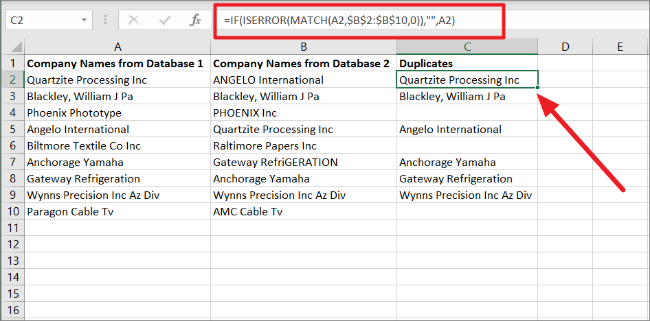
For example, we can use the below formula to compare the two columns and display duplicates in the first column:
=IF(ISERROR(MATCH(A2,$B$2:$B$10,0)),"",A2)Here, the ISERROR function is combined with the IF function to find errors and display text strings or blanks.
The MATCH function searches and returns the position of A2 (in the range B2:B10) as 5. Since it is not an error, the ISERROR function returns FALSE, and the IF function returns the value of A2. In another instance, the MATCH function in C6 returns a #N/A error because the value of A6 is not found in the range B2:B10. Hence, the ISERROR function returns TRUE, and subsequently, the IF function returns the blank.
Display Unique Data using the MATCH function
If you want to compare two columns and display the unique values in each column, you can also do that with the same above formula by simply swapping the last 2 arguments of the IF function.
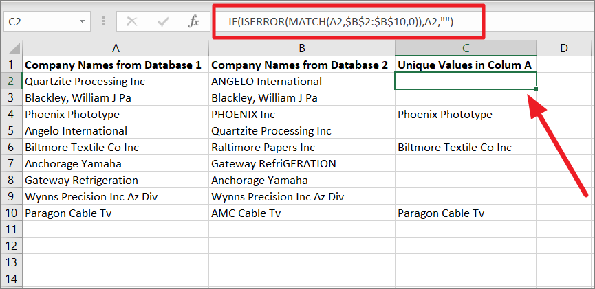
To display unique values in the first column, enter the below formula:
=IF(ISERROR(MATCH(A2,$B$2:$B$10,0)),A2,"")The MATCH function searches and returns the position of A2 (in the range B2:B10) as 5. Since the result is not an error, the ISERROR function returns FALSE and the IF function returns the blank space.
The MATCH function in C4 returns a #N/A error because the value of A4 is not found in the range B2:B10. Hence, the ISERROR function returns TRUE, and subsequently, the IF function returns the value of A4.
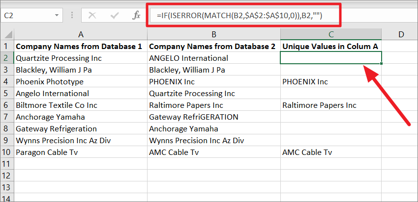
To display unique values in the second column, enter the below formula:
=IF(ISERROR(MATCH(B2,$A$2:$A$10,0)),B2,"")The MATCH function looks at and returns the position of B2 (in the range A2:A10) as 5. Since the result is not an error, the ISERROR function returns FALSE and the IF function returns the blank space.
The MATCH function in C4 returns a #N/A error because the value of B4 is not found in the range B2:B10. Hence, the ISERROR function returns TRUE, and subsequently, the IF function returns the value of B4.
Compare Two Columns using INDEX and MATCH Functions
The MATCH function can be combined with the INDEX function to compare and match two columns. Compared to VLOOKUP, the INDEX MATCH is a powerful and versatile formula that can compare two columns and also pull the matching data.
The INDEX function is used to retrieve a value at a specific location in a table or a range. The MATCH function returns the relative position of a value in a column or a row. When combined, the MATCH finds the row or column number (location) of a specific value, and the INDEX function retrieves a value based on that row and column number.
Syntax of INDEX function:
=INDEX(array,row_num,[col_num],)- array – The arrays of cells in which you are searching for a value.
- row_num – It represents the row in the array from which to return a value. If row_num is omitted, column_num is required.
- column_num – It represents the column in the array from which to return a value. If column_num is omitted, row_num is required.
Example:
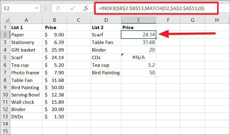
To compare the two columns A and D and fetch the price (the matched value) for column D by using INDEX and MATCH:
=INDEX($B$2:$B$13,MATCH(D2,$A$2:$A$13,0))Enter the formula in cell E2 and copy it down the range E3:E7. Now, let’s see how the formula works:
INDEX function needs a row and column number to retrieve a value. In the above formula, the nested MATCH function finds the row number (position) of the value D2. Then we supply that row number (5) to the INDEX function with a range B2:B13. We specified ‘0’ as the last argument to ignore the column number because we are considering only one column in our array, column B ($B$2:$B$13).
Finally, the INDEX function returns the 5th value in the array B2:B13, which is 24.14.
As you can see, we encountered the #N/A errors in cell E5 because the cell value D5 is not available in column A. To avoid such errors, you can wrap the formula with an IFERROR function.
=IFERROR(INDEX($B$2:$B$13,MATCH(D2,$A$2:$A$13,0)),"")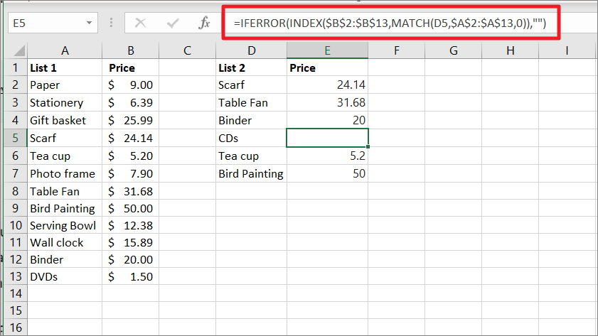
Using Wildcards
In case there is little difference in the names in the two columns that we are comparing, you can partially match columns by adding wildcards to the formula.
Wildcards can be used in the MATCH function only when match_type is set to ‘0’ and the lookup value is a text string. There are wildcards you can use in the MATCH function: an asterisk (*) and a question mark (?).
- Question mark (?) is used to match any single character or letter with the text string.
- Asterisk (*) is used to match any number of characters with the string.
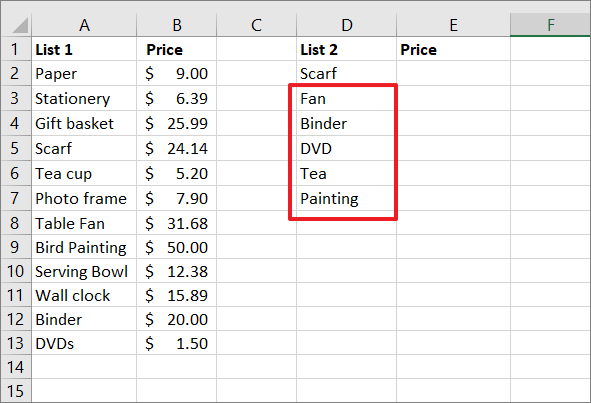
As you can see below, the names in List 2 are not as complete as in List 1, so using wildcards can make up for the missing characters.
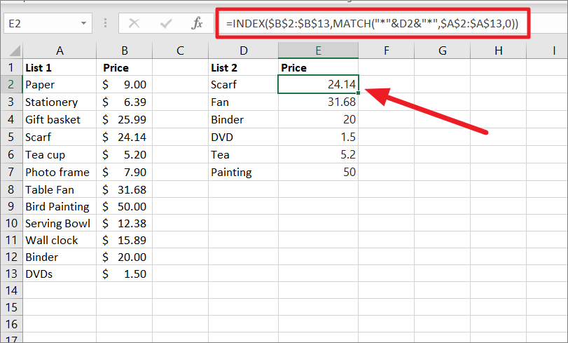
=INDEX($B$2:$B$13,MATCH("*"&D2&"*",$A$2:$A$13,0))In the above formula, D2 has been enclosed in ‘&’ operators and asterisks “*” to make up for the missing character before and after the lookup value. If list 2 doesn’t have the entire name of the items, the asterisks characters will make up for the missing characters and extract values from the partially matched columns.
Compare Two Columns and Find Matches and Differences using VBA Macro
In case you need to compare and match columns often or repeatedly, you can create VBA Macros to automate those tasks. You can use VBA code to create custom user-generated functions to perform tasks and calculations. Here’s how you can do that:
Compare Two Columns Row by Row and Highlight Differences using VBA Code
VBA Macro is the quickest and most effective way to compare two columns in Excel. If you want to compare two columns and highlight the differences between them, follow the instructions:
First, open the workbook that contains the two columns you want to compare.
Then, go to the ‘Developer’ tab and click the ‘Visual Basic’ option from the ribbon or press Alt+F11 keyboard shortcut to open Microsoft Visual Basic for Applications.
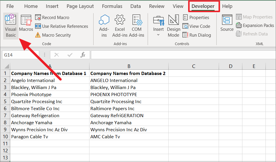
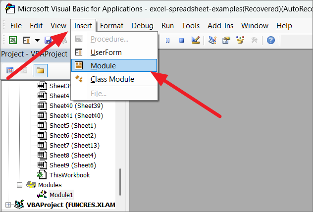
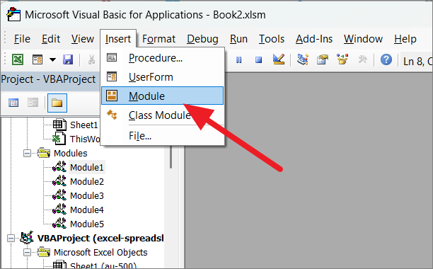
This will open Microsoft Visual Basic for Applications in a separate window. In the VBA window, click the ‘Insert’ menu and select the ‘Module’ option. Alternatively, you can just right-click on the ‘Microsoft Excel Objects’ in the navigation bar on the left, click ‘Insert’, and then select ‘Module’ from the sub-menu.
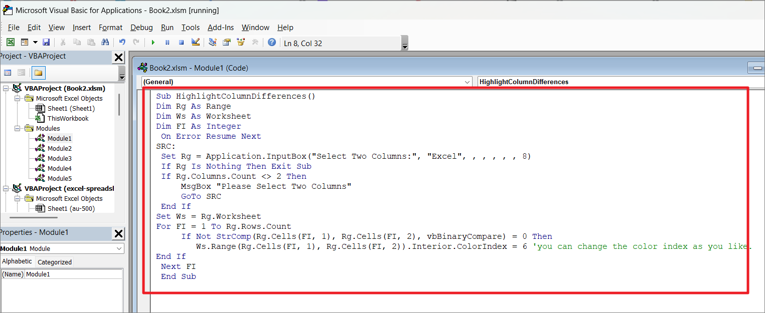
Now, copy and paste the following VBA script into the new module window:
Sub HighlightColumnDifferences()
Dim Rg As Range
Dim Ws As Worksheet
Dim FI As Integer
 On Error Resume Next
SRC:
 Set Rg = Application.InputBox("Select Two Columns:", "Excel", , , , , , 8)
 If Rg Is Nothing Then Exit Sub
 If Rg.Columns.Count <> 2 Then
     MsgBox "Please Select Two Columns"
     GoTo SRC
 End If
Set Ws = Rg.Worksheet
For FI = 1 To Rg.Rows.Count
     If Not StrComp(Rg.Cells(FI, 1), Rg.Cells(FI, 2), vbBinaryCompare) = 0 Then
        Ws.Range(Rg.Cells(FI, 1), Rg.Cells(FI, 2)).Interior.ColorIndex = 6 'you can change the color index as you like.
End If
 Next FI
 End Sub
The above code allows you to compare two columns row by row and highlight the differences between them.
After pasting the script, click ‘File’ and select ‘Save XXXX (filename)’ to save this module as a macro.
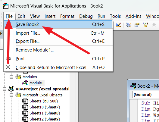
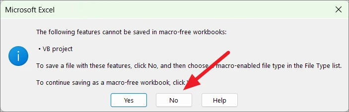
The VB script needs to be saved in a macro-enabled file type. Once you click ‘Save’, you will see a prompt box asking whether you want to save this file in a macro-free file or macro-enabled file type.
Click ‘No’ to choose the macro-enabled file type.
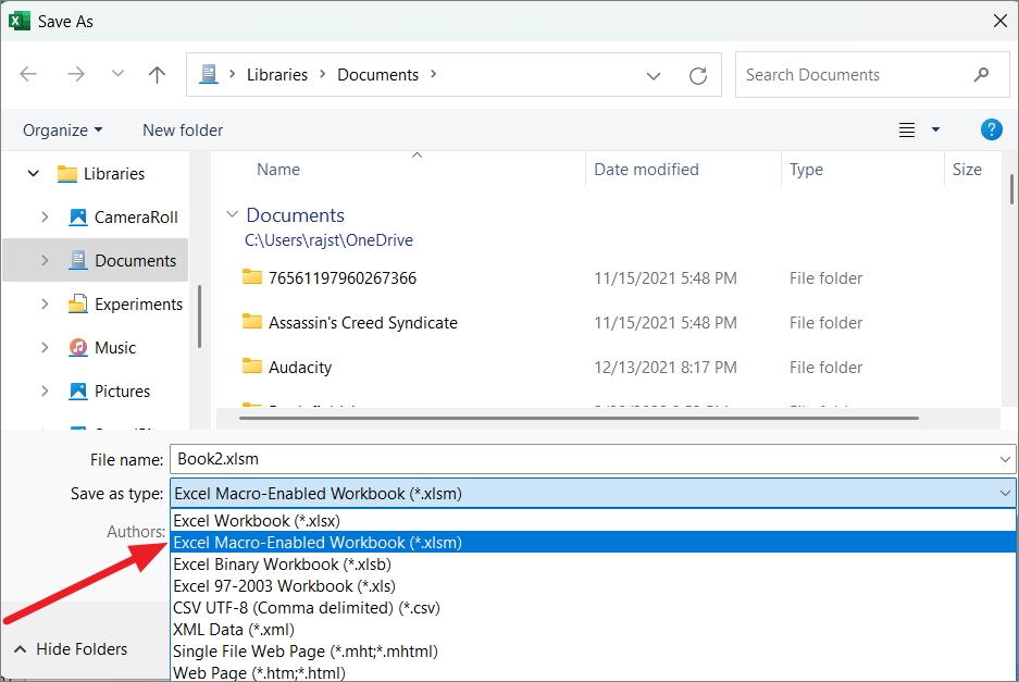
In the Save As window, choose the ‘Excel Macro-Enabled Workbook (*.xlsm)’ format from the ‘Save As type’ drop-down.
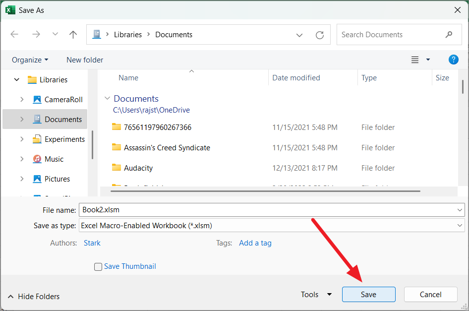
Then, click the ‘Save’ button to save the VBA macro with the workbook.
Now, you can run the macro to compare columns.
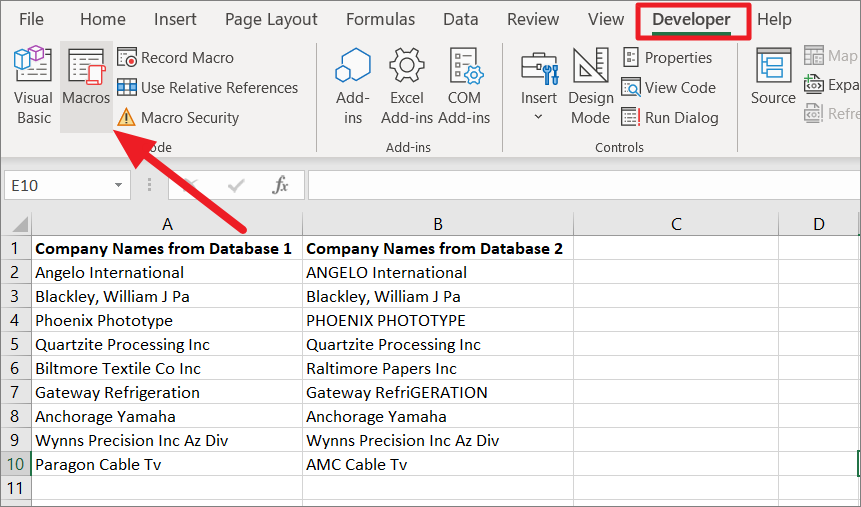
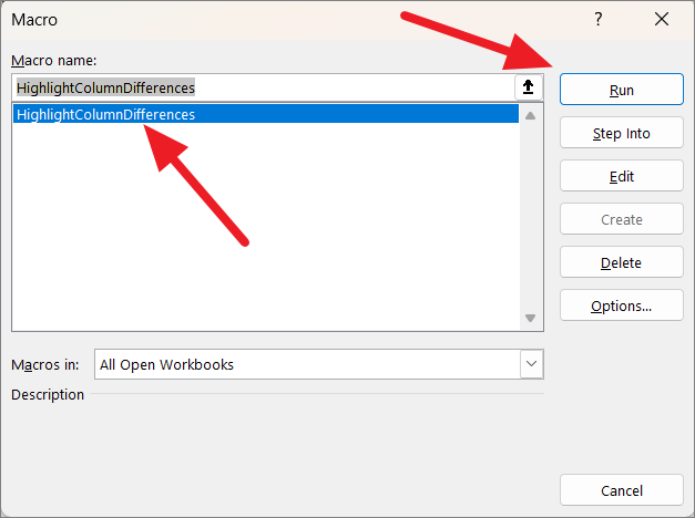
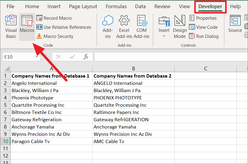
Go back to your Excel worksheet, then head to the ‘Developer’ tab in ‘Ribbon’ and select ‘Macros’ or press ALT+F8.
A dialog box named Macro will open up. Under the Macro name, you will see the macro you created. Select the ‘HighlightColumnDifference’ macro and click ‘Run’.
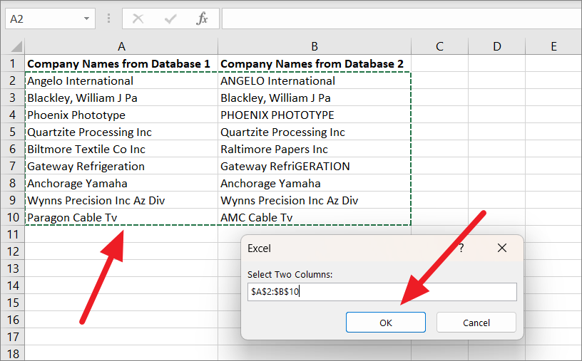
Now, you will see a dialog box for specifying the two columns. Simply select the columns you want to compare and click ‘OK’.
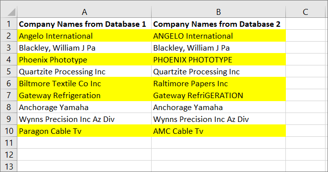
The differences between the two columns will be highlighted with a background color you specified in the code. This VBA code compares columns with case-sensitive and highlights the differences.
Compare Two Columns and Highlight Matching Data (or Duplicates) using VBA Code
If you want to compare two columns and then highlight the matches or duplicates in the second column, you can use the below code.
Open the spreadsheet and press Alt+F11 to open the Microsoft Visual Basic for Applications window. Then, go to ‘Insert’ > ‘Module’ in the Microsoft Visual Basic for Applications window.
Next, copy-paste the below macro code into the new blank Module script:
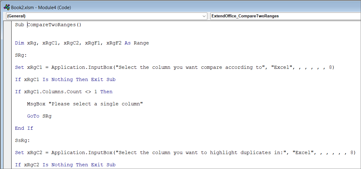
Sub CompareTwoRanges()
Dim xRg, xRgC1, xRgC2, xRgF1, xRgF2 As Range
SRg:
Set xRgC1 = Application.InputBox("Select the column you want compare according to", "Excel", , , , , , 8)
If xRgC1 Is Nothing Then Exit Sub
If xRgC1.Columns.Count <> 1 Then
MsgBox "Please select a single column"
GoTo SRg
End If
SsRg:
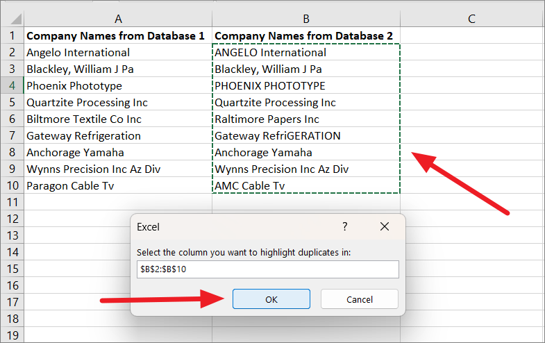
Set xRgC2 = Application.InputBox("Select the column you want to highlight duplicates in:", "Excel", , , , , , 8)
If xRgC2 Is Nothing Then Exit Sub
If xRgC2.Columns.Count <> 1 Then
MsgBox "Please select a single column"
GoTo SsRg
End If
For Each xRgF1 In xRgC1
For Each xRgF2 In xRgC2
If xRgF1.Value = xRgF2.Value Then
xRgF2.Interior.ColorIndex = 38 '(you can change the color index as you need)
End If
Next
Next
End Sub
After pasting the code save the file as a Macro-Enabled Workbook with ‘*.xlsm’ format like we showed you above. Then, close the module and Microsoft Visual Basic for Applications window.
To run the VBA macro, switch to the ‘Developer’ tab and click ‘Macros’ from the Code group.
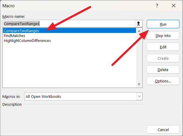
In the Macro dialog window, select ‘CompareTwoRanges’ and click ‘Run’.
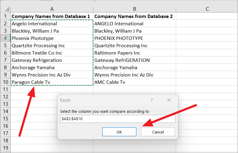
When you see the first pop-up dialog box, select the column that you want to compare duplicate values according to and click ‘OK’.
In the second dialog box, select the column where you want to highlight duplicate values and click ‘OK’.
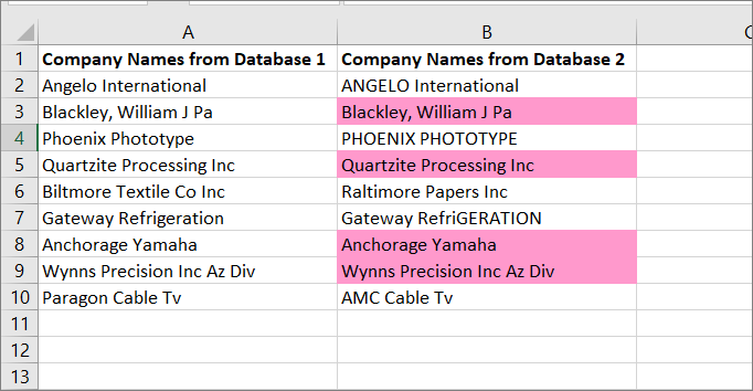
As you can see below, the second column is compared against the first column, and duplicates are highlighted in the second column with a background color. This VBA code compares columns with case-sensitive matches.
Compare Two Columns and Extract Matching Data using VBA Code
In case you want to compare two columns row by row and pull the matching values (duplicates) to another column, you can use the below macro code.
Open a blank module in the Microsoft Visual Basic for Applications window as we showed you. Copy and paste the below script to the new blank module :
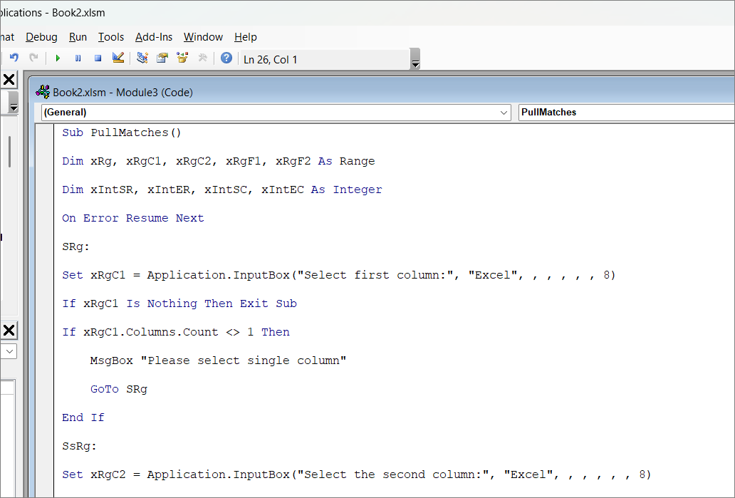
Sub PullMatches()

Dim xRg, xRgC1, xRgC2, xRgF1, xRgF2 As Range

Dim xIntSR, xIntER, xIntSC, xIntEC As Integer

On Error Resume Next

SRg:

Set xRgC1 = Application.InputBox("Select first column:", "Excel", , , , , , 8)

If xRgC1 Is Nothing Then Exit Sub

If xRgC1.Columns.Count <> 1 Then

    MsgBox "Please select single column"

    GoTo SRg

End If

SsRg:

Set xRgC2 = Application.InputBox("Select the second column:", "Excel", , , , , , 8)

If xRgC2 Is Nothing Then Exit Sub

If xRgC2.Columns.Count <> 1 Then

    MsgBox "Please select single column"

    GoTo SsRg

End If

Set xWs = xRg.Worksheet


For FI = 1 To xRg.Rows.Count
     If Not StrComp(xRg.Cells(FI, 1), xRg.Cells(FI, 2), vbBinaryCompare) = 0 Then
        Ws.Range(xRg.Cells(FI, 1), Rg.Cells(FI, 2)).Interior.ColorIndex = 8 'you can change the color index as you like.
End If
 Next FI

End Sub
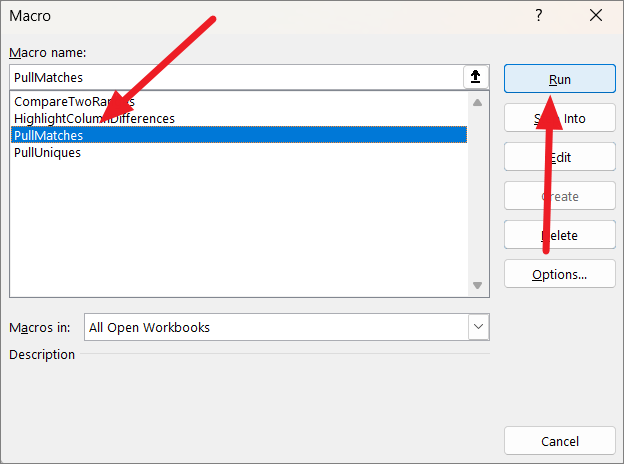
After pasting the code save the file and close the Microsoft Visual Basic for Applications window. Then, open the Marco dialog window, select the ‘PullMatches’ macro and click ‘Run’.
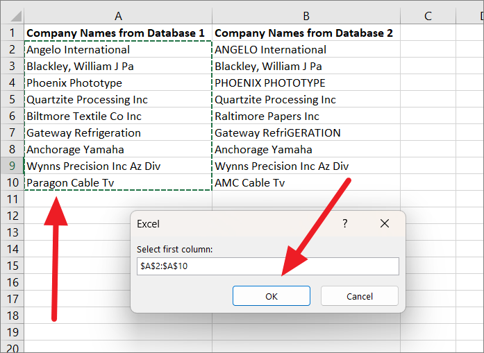
First, select the first column (left) you want to compare and click ‘OK’.
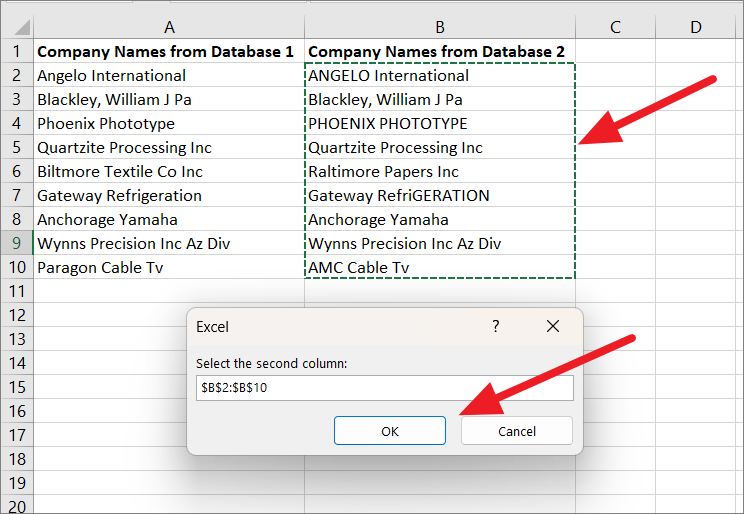
In the second dialog, select the second column you want to compare and click ‘OK’.
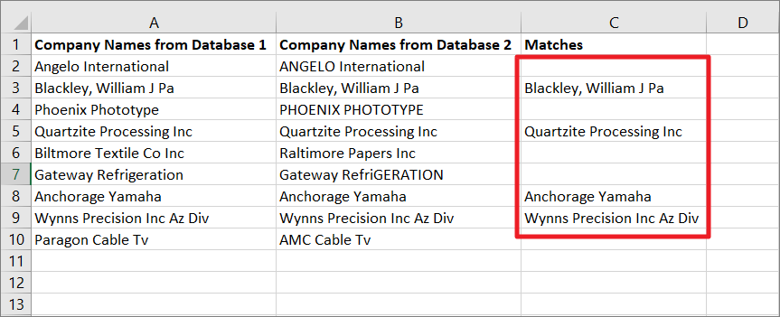
The matches between two columns will be pulled and displayed automatically in the right column of the two columns you selected.
Compare Two Columns and Extract Unique Data using VBA Code
If you want to two compare columns and pull unique values, here’s the below VBA code that can help you.
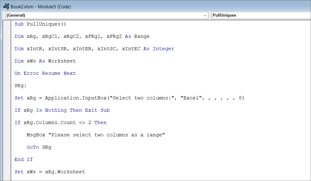
Open a blank module in the Microsoft Visual Basic for Applications window and copy-paste the below script to the new blank module :
Sub PullUniques()

Dim xRg, xRgC1, xRgC2, xFRg1, xFRg2 As Range

Dim xIntR, xIntSR, xIntER, xIntSC, xIntEC As Integer

Dim xWs As Worksheet

On Error Resume Next

SRg:

Set xRg = Application.InputBox("Select two columns:", "Excel", , , , , , 8)

If xRg Is Nothing Then Exit Sub

If xRg.Columns.Count <> 2 Then

    MsgBox "Please select two columns as a range"

    GoTo SRg

End If

Set xWs = xRg.Worksheet


xIntSC = xRg.Column

xIntEC = xRg.Columns.Count + xIntSC - 1

xIntSR = xRg.Row

xIntER = xRg.Rows.Count + xIntSR - 1


Set xRg = xRg.Columns

Set xRgC1 = xWs.Range(xWs.Cells(xIntSR, xIntSC), xWs.Cells(xIntER, xIntSC))

Set xRgC2 = xWs.Range(xWs.Cells(xIntSR, xIntEC), xWs.Cells(xIntER, xIntEC))

xIntR = 1

For Each xFRg In xRgC1

    If WorksheetFunction.CountIf(xRgC2, xFRg.Value) = 0 Then

        xWs.Cells(xIntER, xIntEC).Offset(xIntR) = xFRg

        xIntR = xIntR + 1

    End If

Next

xIntR = 1

For Each xFRg In xRgC2

    If WorksheetFunction.CountIf(xRgC1, xFRg) = 0 Then

        xWs.Cells(xIntER, xIntSC).Offset(xIntR) = xFRg

        xIntR = xIntR + 1

    End If

Next

End Sub
Then save the file and close the Microsoft Visual Basic for Applications window.
After that, open the Marco dialog window, select the ‘PullUniques’ macro, and click ‘Run’.
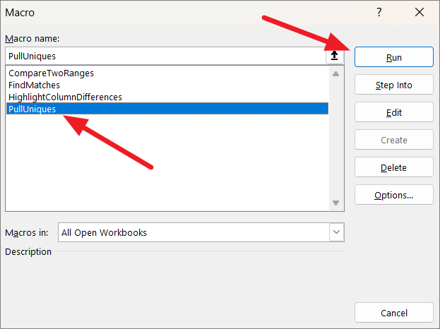
In the pop-up window, select the two comparing columns and click ‘OK’.
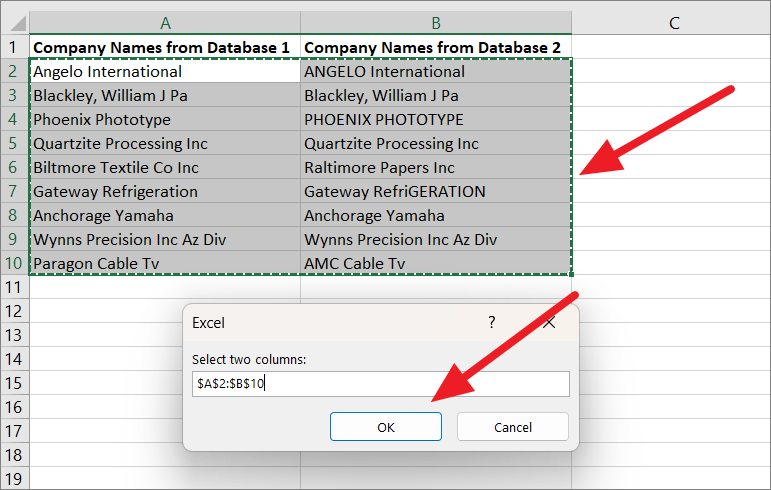
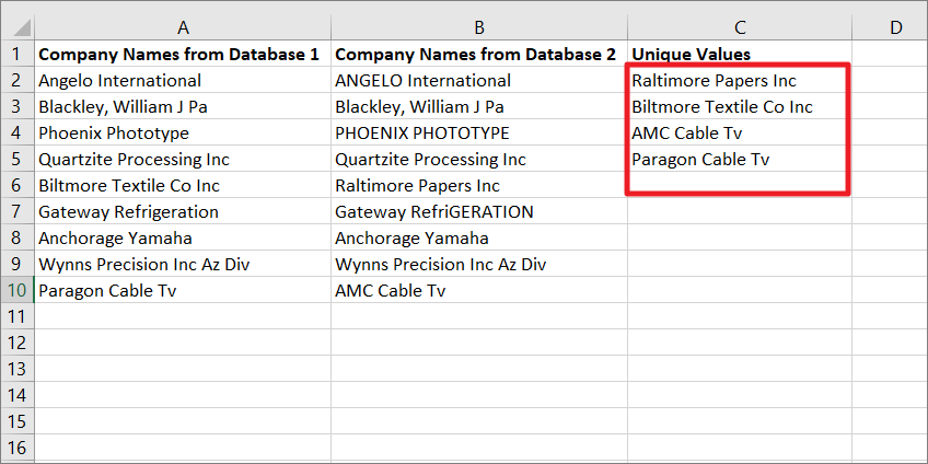
The Macro compares columns without case sensitivity and lists unique values from the two columns.
That’s it. Now, you know everything about comparing columns in Excel. You can opt for the method that suits you the best.


